Dynamic programming
Dynamic Programming:
- breaks a problem down into sub-problems
- solves them
- saves the results
- and then uses these sub-results to compute the larger result
This process can be naturally done either with:
- recursion + memoization (top-down decomposition)
- iteration + tabulation (bottom-up composition)
It’s applicable where the nature of a problem is that:
-
there are overlapping subproblems (i.e., same subproblem appears multiple times) that it can avoid recomputing
-
optimal substructure: its optimal solution can be found by combining the results of optimal solutions to sub-problems.
Conceptually, DP is like “optimized recursion via caching.” Morally, it’s like brute force + memoization. It just works really well when it applies (when the two conditions hold), so we can structure our computation correctly and cache.
Backtracking
Backtracking is a recursive search algorithm that incrementally builds partial solutions and abandons paths that cannot become full solutions.
Additional notes:
- by nature recursive; could implement iteratively with a stack
- morally, it’s like brute force + pruning
One example is the N-queens problem.
Click to show Backtracking N-Queens in Python
"""backtracking, trying the N queens problem. more:
- https://en.wikipedia.org/wiki/Backtracking
- https://en.wikipedia.org/wiki/Eight_queens_puzzle

takeaways from backtracking:

1.  I always called the technique  "recursive backtracking", but most just
    call it "backtracking" because recursion is so commonly used. (could do
    iter + stack if wanted.)

2. backtracking feels morally similar to brute force. (still seems exponential
   or super-exponential.) though cutting off whole search subtrees is
   undoubtedly good. (e.g., if can't place 6th queen from these 5, no need to
   also try placing 7th and 8th)

3. even simple heuristics dramatically reduce search space. for example,
   knowing there's 1 queen per row, so searching row-by-row, enormously
   reduces the search space.

some things i learned with display: - clearing screen is really easy - seeing
the attempts is really fun - doing so makes attempts 2-3 ORDERS OF MAGNITUDE
slower
    - e.g., 300 vs 270,000 attempts per second
- as always, measure before optimizing is good
    - (this i/o bound was sufficient to remove for what i wanted to try)

better implementations would probably use bitmaps and vector ops to check
row/col/diag collisions, rather than iterating like I do here

one surprising thing is that stupider searching (trying each queen placement
from [0][0] through [n][n]) checks 4x attempts/second vs smarter search
(automatically assigning queen i to row i, and only searching [i][0] through
[i][n])
"""

import os
import time
from typing import Optional

attempt = 0

last_reported = time.time()
attempts_since_last_report = 0
report_interval_s = 1


def render(board_size: int, queens: set[tuple[int, int]]):
    global attempt
    attempt += 1
    for row in range(board_size):
        buf = []
        for col in range(board_size):
            if (row, col) in queens:
                buf.append("[Q]")
            else:
                buf.append("[ ]")
        print("".join(buf))
    print(f"{len(queens)} queens (attempt {attempt})")


def render_lite(board_size: int, queens: set[tuple[int, int]]):
    global attempt, last_reported, attempts_since_last_report
    attempt += 1
    attempts_since_last_report += 1
    now = time.time()
    delta = now - last_reported
    if delta > report_interval_s:
        last_reported = now
        clear()
        aps = int(attempts_since_last_report / delta)
        attempts_since_last_report = 0
        print(
            f"attempt {attempt} (@{len(queens)}/{board_size} queens) ({aps} attempts/s)"
        )


def clear():
    os.system("cls" if os.name == "nt" else "clear")
    # print()
    pass


def tick():
    # time.sleep(0.01)
    pass


def collides(board_size: int, queens: set[tuple[int, int]]):
    for queen in queens:
        in_row = len([q for q in queens if q[0] == queen[0]])
        if in_row > 1:
            # print(f"{queen} collides row {queen[0]}")
            return True
        in_col = len([q for q in queens if q[1] == queen[1]])
        if in_col > 1:
            # print(f"{queen} collides col {queen[1]}")
            return True
        # 2 diagonal checks.
        # (1) UL --> BR
        r, c = queen
        n_ulbr = 0
        while r >= 0 and c >= 0:
            if (r, c) in queens:
                n_ulbr += 1
            r -= 1
            c -= 1
        r, c = queen[0] + 1, queen[1] + 1
        while r < board_size and c < board_size:
            if (r, c) in queens:
                n_ulbr += 1
            r += 1
            c += 1
        if n_ulbr > 1:
            # print(f"{queen} collides UL -> BR")
            return True
        # (1) BL --> UR
        # - to BL: rows increase, columns decrease
        r, c = queen
        n_blur = 0
        while r < board_size and c >= 0:
            if (r, c) in queens:
                n_blur += 1
            r += 1
            c -= 1
        # - to UR: rows decrease, columns increase
        r, c = queen[0] - 1, queen[1] + 1
        while r >= 0 and c < board_size:
            if (r, c) in queens:
                # print(f"({r}, {c}) in queens")
                n_blur += 1
            r -= 1
            c += 1
        if n_blur > 1:
            # print(f"{queen} collides BL -> UR")
            return True
    return False


def test_collides():
    assert collides(8, set([(0, 0), (0, 1)]))
    assert collides(8, set([(0, 0), (1, 0)]))
    assert collides(8, set([(0, 0), (1, 1)]))

    assert collides(8, set([(7, 7), (7, 0)]))
    assert collides(8, set([(7, 7), (7, 6)]))
    assert collides(8, set([(7, 7), (0, 7)]))
    assert collides(8, set([(7, 7), (6, 7)]))
    assert collides(8, set([(7, 7), (0, 0)]))

    assert collides(8, set([(3, 3), (2, 2)]))
    assert collides(8, set([(3, 3), (4, 4)]))
    assert collides(8, set([(3, 3), (4, 2)]))
    assert collides(8, set([(3, 3), (2, 4)]))

    assert not collides(8, set([(0, 0), (1, 2)]))
    assert not collides(8, set([(0, 0), (2, 1)]))
    assert not collides(8, set([(0, 0), (2, 3)]))


def place_queen_naive(
    board_size: int, queens: set[tuple[int, int]]
) -> Optional[set[tuple[int, int]]]:
    """with rendering, this checked like ~300 attempts per second, which is hilariously
    low"""
    # print(f"place_queen(board_size={board_size}, queens={len(queens)})")
    # base case: we're done when we've placed board_size queens
    if len(queens) == board_size:
        return queens
    # brute force w/ .... backtracking?
    for r in range(board_size):
        for c in range(board_size):
            if (r, c) in queens:
                continue
            attempt = queens | {(r, c)}

            # ~300 aps
            # tick()
            # clear()
            # render(board_size, attempt)

            # ~270,000 aps
            render_lite(board_size, attempt)

            if not collides(board_size, attempt):
                # attempt is viable, so proceed
                continuation = place_queen_naive(board_size, attempt)
                if continuation is not None:
                    return continuation  # full solution
                # otherwise, we just continue (loops to next C)
    return None


def place_queen_byrow(
    board_size: int, queens: set[tuple[int, int]]
) -> Optional[set[tuple[int, int]]]:
    """with rendering, this checked like ~300 attempts per second, which is hilariously
    low"""
    # print(f"place_queen(board_size={board_size}, queens={len(queens)})")
    # base case: we're done when we've placed board_size queens
    if len(queens) == board_size:
        return queens
    # by row, still brute force w/ .... backtracking?
    r = len(queens)  # 1 queen / row (else trivial collision)
    for c in range(board_size):
        if (r, c) in queens:
            continue
        attempt = queens | {(r, c)}

        # ~300 aps
        # tick()
        # clear()
        # render(board_size, attempt)

        # ~70,000 aps
        render_lite(board_size, attempt)

        if not collides(board_size, attempt):
            # attempt is viable, so proceed
            continuation = place_queen_byrow(board_size, attempt)
            if continuation is not None:
                return continuation  # full solution
            # otherwise, we just continue (loops to next C)
    return None


def main() -> None:
    test_collides()

    # placements = place_queen_naive(8, set())  # solution @ 1,502,346
    # placements = place_queen_byrow(8, set())  # few seconds, solution @ 876
    placements = place_queen_byrow(20, set())  # ~1min, solution @ 3,992,511
    if placements is not None:
        render(len(placements), placements)
    print(f"Complete, result was: {placements}")

    # board_size = 8
    # clear()
    # render(board_size, set([(1, 2), (7, 7)]))
    # tick()
    # clear()
    # render(board_size, set([(0, 0), (0, 7)]))


if __name__ == "__main__":
    main()
From my source repo.
Prefix Sum
AKA: cumulative sum, scan.
One of those buzzwords I should probably know, the prefix sum y of an array x is simply the element-wise cumulative sum, so y[i] = sum(x[:i+1]) (i.e., inclusive).
Click to show Prefix Sum in Python
"""AKA cumulative sum, scan.

For an input array x, its prefix sum is a new array y, where each entry y[i]
is the cumulative sum of x from x[0] through x[i].
"""

prefix_sum_oneliner = lambda x: [sum(x[:i]) for i in range(len(x))]
"""cute O(n^2) prefix sum that's a python one-liner."""


def prefix_sum(xs: list[int]) -> list[int]:
    """Returns prefix sum of xs in O(n)."""
    y = [0] * len(xs)
    for i, x in enumerate(xs):
        y[i] = x + (y[i - 1] if i > 0 else 0)
    return y


def main() -> None:
    a = [1, 2, 3, 4, 5]
    b = prefix_sum(a)
    print(a)
    print(b)


if __name__ == "__main__":
    main()
From my source repo.
Maximum sum sub-array
Kadane’s Algorithm finds the maximum sum sub-array of an array in O(n).
In short, you:
- track both the best sum seen and the current sum
- the current sum is reset whenever an element alone is better than continuing it
- (and just keep updating the best sum seen)
The key for doing this in one pass is the surprising intuition that the current sum c can be reset to just the present element x if x > x + c. In other words, if the current sum is negative, it’s always better to just start over at the current position than carry the negative baggage onwards.
The exception you might imagine is if you have just a single negative element, with positive elements on both sides ([+ - +]). You’d get a great sum by spanning the negative element to include both positive ones, so are you sure you want to reset? The answer is: yes, because just using the last element (x) is greater than all three (x + c).
The implementation is blissfully concise when not tracking indices, and a bit more annoying when tracking indices (which it seems like you’d want to do in any useful application.).
Click to show Kadane's Algorithm for maximum sum sub-array in Python
"""Kadane's algorithm for finding the maximum sum sub-array in O(n)."""

from typing import Optional


def kadane_no_indices(xs: list[int]) -> Optional[int]:
    """easy mode: just returns best sum (or None if empty)"""
    best_sum, cur_sum = None, 0
    for x in xs:
        cur_sum = max(cur_sum + x, x)  # continue or restart
        best_sum = max(best_sum, cur_sum) if best_sum is not None else cur_sum
    return best_sum


def kadane(xs: list[int]) -> tuple[int, int, Optional[int]]:
    """returns (best_start, best_end (inclusive!), best_sum | None if empty)"""
    cur_start, cur_end = 0, 0
    best_start, best_end = 0, 0
    cur_sum = 0
    best_sum = None
    for i, x in enumerate(xs):
        if x > cur_sum + x:
            # starting new
            cur_start = i
            cur_end = i
            cur_sum = x
        else:
            # continue sum
            cur_sum = cur_sum + x
            cur_end = i

        # if new best, also update saved indices
        if best_sum is None or cur_sum > best_sum:
            best_start = cur_start
            best_end = cur_end
            best_sum = cur_sum

    return best_start, best_end, best_sum


def main() -> None:
    a = [-2, 1, -3, 4, -1, 2, 1, -5, 4]
    best_start, best_end, best_sum = kadane(a)
    print(a)
    print(f"best: sum(a[{best_start}:{best_end}]) (inclusive)")
    print(f"    = sum({a[best_start : best_end + 1]})")
    print(f"    = {sum(a[best_start : best_end + 1])}")
    print(f"    = {best_sum}")
    print(f"    = {kadane_no_indices(a)}")


if __name__ == "__main__":
    main()
From my source repo.
Quicksort
Quicksort:
- choose pivot element
- partition into < and > the pivot
- put pivot right at that boundary
- quicksort each partition
Key properties:
- worst case: O(n^2)
- average case: O(n log n)
- in-place
- space: O(log n) b/c you gotta have a O(log n) call stack
- wikipedia says you gotta use “Sedgewick’s trick” to sort the larger partition using tail recursion or iteration, else you might use O(n) recursive calls. hmm.
Quicksort’s degenerate case is on an already sorted array:
- say we choose the pivot to be the last element
- the “< pivot” boundary moves from 0 to the last element (O(n))
- then, the left partition has n-1 elements, and the right partition is empty
- we quicksort the left partition, which happens O(n) times recursively
Click to show a heavily-commented Quicksort in Python
"""Quicksort:
- choose pivot element
- partition into < and > the pivot
- put pivot right at that boundary
- quicksort each partition

Key properties:
- worst case: O(n^2)
- average case: O(n log n)
- in-place
- space: O(log n) b/c you gotta have a O(log n) call stack
    - wikipedia says you gotta use "Sedgewick's trick" to sort the larger
      partition using tail recursion or iteration, else you might use O(n)
      recursive calls. hmm.

Quicksort's degenerate case is on an already sorted array:
- say we choose the pivot to be the last element
- the "< pivot" boundary moves from 0 to the last element (O(n))
- then, the left partition has n-1 elements, and the right partition is empty
- we quicksort the left partition, which happens O(n) times recursively
"""

import random


def quicksort(x: list[int], start: int = 0, end: int = -1) -> None:
    """in-place quicksorts x from start through end, both inclusive."""
    if end == -1:
        end = len(x) - 1

    # base case: any sequence of 0 or 1 (or negative, lol) elements is sorted
    if start >= end:
        return

    # conceptual notes:
    # - boundary is inclusive
    # - i >= boundary, i.e., we'll iterate at least as fast as the boundary grows
    # - we compare up to pivot (exclusive)
    pivot = x[end]  # subject of comparison
    boundary = start - 1  # invariant: all els <= boundary will be <= pivot
    for i in range(start, end):
        if x[i] <= pivot:
            # if x[i] <= pivot, it should live in the left (<= boundary)
            # region. we can accomplish this by:
            # - extending the boundary by one to accommodate it, then
            # - swapping it with whatever is there. this is ok b/c:
            #      - conceptually, we're swapping left (i >= boundary)
            #      - so either now i == boundary (and swap is noop),
            #      - or i > boundary, and what we're swapping x[i] with at
            #        x[boundary] has already been checked, and is > pivot
            #        anyway, so it's fine staying right of the boundary, moving
            #        potentially much further right to wherever x[i] is
            boundary += 1
            x[i], x[boundary] = x[boundary], x[i]
        else:
            # x[i] > pivot, so it should live right of the boundary. this is
            # fine, we just keep boundary where it is.
            pass

    # now, we have two partitions, and the pivot:
    # x[start : boundary + 1] (i.e., boundary-inclusive) that's <= pivot
    # x[boundary + 1 : end] (i.e., pivot-exclusive) that's > pivot
    # x[end] the pivot
    #
    # if we swap the pivot into right after the boundary, it'll live at the right place.
    # (bounds ok? yes: boundary is at most the same as end.)
    x[end], x[boundary + 1] = x[boundary + 1], x[end]

    # now the partitions and the pivot are at:
    # x[start : boundary + 1]  <-- <= pivot
    # x[boundary + 1]          <-- pivot
    # x[boundary + 2 : end]    <-- > pivot
    #
    # we quicksort the partitions
    quicksort(x, start, boundary)  # not `boundary + 1`, b/c inclusive
    quicksort(x, boundary + 2, end)  # boundary + 2 ok? just check in call


def main() -> None:
    n = 10
    x = random.sample(range(1, n + 1), n)
    print(f"Before: {x}")
    quicksort(x)
    print(f"After:  {x}")
    assert x == sorted(x)


if __name__ == "__main__":
    main()
From my source repo.
Mergesort
Mergesort:
- divide
- conquer (sort)
- merge (easy b/c sorted)
Properties:
- best O(n log n)
- worst O(n log n)
- in general, not in-place;
- in general, needs O(n) extra space
Click to show Mergesort in Python
"""Mergesort

- divide
- conquer (sort)
- merge (easy b/c sorted)

Properties:
- best O(n log n)
- worst O(n log n)
- in general, not in-place;
- in general, needs O(n) extra space
"""

import random


def mergesort(x: list[int]) -> list[int]:
    # 0- or 1-el lists are sorted
    if len(x) <= 1:
        return x

    # divide. as with all binary stuff, OBOB easy to do.
    # n    n // 2   x[:middle], x[middle:]
    # ---  ---      ---
    # 0     0       n/a! would have returned
    # 1     0       n/a! would have returned
    # 2     1       [0], [1]
    # 3     1       [0], [1,2]
    # 4     2       [0,1], [2,3]
    # 5     2       [0,1], [2,3,4]
    # ...
    middle = len(x) // 2

    # conquer
    left = mergesort(x[:middle])
    right = mergesort(x[middle:])

    # merge
    sorted = []
    i, j = 0, 0
    while i < len(left) or j < len(right):
        # if either list is exhausted, add rest from the other. (might as well
        # do all at once.)
        if i == len(left):
            sorted.extend(right[j:])
            j = len(right)
        elif j == len(right):
            sorted.extend(left[i:])
            i = len(left)
        else:
            # standard case, we add whichever is smaller
            if left[i] < right[j]:
                sorted.append(left[i])
                i += 1
            else:
                sorted.append(right[j])
                j += 1
    return sorted


def main() -> None:
    n = 10
    x = random.sample(range(1, n + 1), n)
    print(f"Before: {x}")
    sorted_x = mergesort(x)
    print(f"After:  {sorted_x}")
    assert sorted_x == sorted(x)


if __name__ == "__main__":
    main()
From my source repo.
Binary Tree
For the searches below, we’ll use a simple generic binary tree (node) implementation, roughly:
class TreeNode(Generic[T]):

    def __init__(
        self,
        val: Optional[T] = None,
        left: Optional["TreeNode"] = None,
        right: Optional["TreeNode"] = None,
    ):
        self.val = val
        self.left = left
        self.right = right
There’s also a convenience build() method which takes a list of nodes in array representation, assumes it is formatted as a complete binary tree (i.e., top-down layer traversal, left-right within layers), and builds a tree from it. Empty spots in the tree (None) are fine, as long as they aren’t parents
The full implementation, including build(), is below.
Click to show a generic binary tree node implementation in Python
r"""Minimal generic binary tree (node) used in both DFS and BFS.

TreeNode.build() builds an array from a complete binary tree
representation. `None`s are fine, just not as parents.
Using 0-based indexing.

           0
        /     \
      1          2
    /  \       /   \
   3    4     5     6
  / \  / \   / \   / \
 7  8 9 10  11 12 13 14

node i,'s children are:
    left: i*2 + 1
    right: i*2 + 2
"""

from typing import Generic, TypeVar, Optional

T = TypeVar("T")


class TreeNode(Generic[T]):
    __slots__ = ("val", "left", "right")

    def __init__(
        self,
        val: Optional[T] = None,
        left: Optional["TreeNode"] = None,
        right: Optional["TreeNode"] = None,
    ):
        self.val = val
        self.left = left
        self.right = right

    def __repr__(self) -> str:
        l = self.left.val if self.left is not None else "None"
        r = self.right.val if self.right is not None else "None"
        return f"TreeNode({self.val}, L={l}, R={r})"

    @staticmethod
    def build(complete: list[Optional[T]]) -> "TreeNode[T]":
        """Returns root or errors if not possible (just to minimize None checks)."""
        if len(complete) == 0 or complete[0] is None:
            raise ValueError(f"Must pass root. Complete was: {complete}")

        root = TreeNode(complete[0])
        flat_nodes: list[Optional["TreeNode[T]"]] = [None] * len(complete)
        for i, val in enumerate(complete):
            if i == 0:
                flat_nodes[0] = root
                continue
            if val is None:
                continue
            parent_idx = (i - 1) // 2
            parent = flat_nodes[parent_idx]
            if parent is None:
                raise ValueError(
                    f"Node {i} ({val})'s parent {parent_idx} must exist, but was None"
                )
            node = TreeNode(val=val)
            if (parent_idx * 2) + 1 == i:
                parent.left = node
            else:
                assert (parent_idx * 2) + 2 == i
                parent.right = node
            flat_nodes[i] = node
        return root


def main() -> None:
    root = TreeNode.build(list(range(15)))
    print("root:", root)


if __name__ == "__main__":
    main()
From my source repo.
DFS: Depth-First Search
Depth-first search allows:
- natural recursive and iterative (stack) implementations
- different order traversals, which ask the question: when do I visit myself relative to my subtrees?
Click to show depth-first search in Python
r"""DFS: Depth-first search.

Using 0-based indexing.

           0
        /     \
      1          2
    /  \       /   \
   3    4     5     6
  / \  / \   / \   / \
 7  8 9 10  11 12 13 14

node i,'s children are:
    left: i*2 + 1
    right: i*2 + 2

DFS order traversal use cases:

- pre-order:  renders topologically sorted (for every edge (u,v), u comes before v).
              good for copying tree. also, prefix notation.

- in-order:   renders a BST in sorted order

- post-order: render postfix notation (e.g., if internal operators & leaf values).
              also good for deleting tree (removes children first).
"""

from typing import Literal, Optional

from binary_tree import TreeNode, T

Order = Literal["pre", "in", "post"]
ALL_ORDERS: list[Order] = ["pre", "in", "post"]


def dfs_recursive_v1(
    node: TreeNode[T],
    order: Order,
    results: Optional[list[Optional[T]]] = None,
) -> list[Optional[T]]:
    """DFS, depth-first, recursive, kind of gross v1 mutating implementation

    I passed `results` as mutable state into recursive calls. I think
    this is less elegant than using what's returned by the recursion
    as the result.
    """
    # We default argument None, not [], b/c otherwise the default gets mutated!
    if results is None:
        results = []

    if order == "pre":
        results.append(node.val)

    if node.left is not None:
        # NOTE: No need to assign or extend, because
        # - assign? no, we're passing `results` which gets mutated
        # - extend? no, each node's traversal adds itself, so no need to multi-add
        dfs_recursive_v1(node.left, order, results)

    if order == "in":
        results.append(node.val)

    if node.right is not None:
        dfs_recursive_v1(node.right, order, results)

    if order == "post":
        results.append(node.val)

    return results


def dfs(node: Optional[TreeNode[T]]) -> list[Optional[T]]:
    """DFS, depth-first, minimal pure recursive implementation (pre-order)."""
    if node is None:
        return []
    return [node.val, *dfs(node.left), *dfs(node.right)]


def dfs_recursive(
    node: Optional[TreeNode[T]], order: Order
) -> list[Optional[T]]:
    """DFS, depth-first, any-order recursive implementation."""
    if node is None:
        return []
    return [
        *([node.val] if order == "pre" else []),
        *dfs_recursive(node.left, order),
        *([node.val] if order == "in" else []),
        *dfs_recursive(node.right, order),
        *([node.val] if order == "post" else []),
    ]


def dfs_i(root: TreeNode[T]) -> list[Optional[T]]:
    """DFS, depth-first, minimal iterative implementation (pre-order)"""
    res: list[Optional[T]] = []
    stack: list[Optional[TreeNode[T]]] = [root]
    while len(stack) > 0:
        node = stack.pop()
        if node is None:
            continue
        res.append(node.val)
        stack.append(node.right)
        stack.append(node.left)

    return res


def dfs_iterative(root: TreeNode[T], order: Order) -> list[Optional[T]]:
    """DFS, depth-first, iterative

    we add values back to the stack to control the traversal order. this two-pass
    approach lets us decide explicitly when to extract a node's value.
    """
    results = []
    stack: list[TreeNode[T] | Optional[T]] = [root]
    while len(stack) > 0:
        node_or_value = stack.pop()

        # we allow None to simplify adding vals (Optional[T])
        if node_or_value is None:
            continue

        # if we got a value on the stack, that means we should add it
        # to the results.
        if not isinstance(node_or_value, TreeNode):
            val = node_or_value
            results.append(val)
            continue

        # remember to add things "backwards" because stack will pop latest first
        node = node_or_value
        if order == "post":
            stack.append(node.val)
        if node.right is not None:
            stack.append(node.right)
        if order == "in":
            stack.append(node.val)
        if node.left is not None:
            stack.append(node.left)
        if order == "pre":
            stack.append(node.val)
    return results


def main() -> None:
    root = TreeNode.build(list(range(15)))

    # DFS - depth-first
    for order in ALL_ORDERS:
        recursive_v1 = dfs_recursive_v1(root, order)
        recursive = dfs_recursive(root, order)
        iterative = dfs_iterative(root, order)
        assert recursive_v1 == recursive
        assert recursive == iterative
        print(f"DFS ({order}):", recursive)

    # also check the minimal implementations are correct
    assert dfs(root) == dfs_recursive(root, "pre")
    assert dfs_i(root) == dfs_recursive(root, "pre")


if __name__ == "__main__":
    main()
From my source repo.
Order Traversals
The orders are as follows, with “left” standing for “whole left subtree” (& “right” ibid.):
- pre-order: self, left, right
- in-order: left, self, right
- post-order: left, right, self
I love this diagram of when traversals happen in a DFS:
Red = pre, green = in, blue = post. Source: Public Domain via Wikipedia.
There are some applications for each DFS traversal order:
-
Pre-order: renders topologically sorted (for every edge (u,v), u comes before v). Good for copying tree. Also, prefix notation.
-
In-order: renders a BST in sorted order.
-
Post-order: render postfix notation (e.g., if internal operators & leaf values). Also good for deleting tree (removes children first).
Order and Serialization
Consider tree serialization. Perhaps surprisingly, if you use nulls, only pre/post order traversals unambiguously render the tree. In-order traversals are ambiguous, because a parent’s position depends on its subtrees.
| order | unambiguous serialization with nulls? |
|---|---|
| pre | yes |
| in | no |
| post | yes |
Both of the following two binary trees have an in-order traversal of [null, A, null, B, null]:
Tree 1:    B          Tree 2:      A
          /                         \
         A                           B
What if you don’t have nulls? Pre- and post-order traversals no longer unambiguously serialize a tree. But if you have pre + in, or post + in, you can do it. There are even leetcode problems for this:
w/o nulls: pre + in → tree https://leetcode.com/problems/construct-binary-tree-from-preorder-and-inorder-traversal/description/
w/o nulls: in + post → tree https://leetcode.com/problems/construct-binary-tree-from-inorder-and-postorder-traversal/description/
What about pre + post (still no nulls)? It’s not enough. When a node has one child, you can’t tell where it is.
Tree 1:    1          Tree 2:    1
          /                       \
         2                         2
For both:
- pre:
[1, 2] - post:
[2, 1]
BFS: Breadth-First Search
Breadth-first search traverses in complete-tree-as-array order (top to bottom by level, and left to right within each level).
Breadth-first search really only lends itself naturally to an iterative implementation with a queue.
- no recursion: doesn’t have a natural recursive implementation
- no order: doesn’t really have different order traversals (could do right before left, which reverses the within-level order)
Click to show breadth-first search in Python
r"""BFS: Breadth-first search.

Using 0-based indexing.

           0
        /     \
      1          2
    /  \       /   \
   3    4     5     6
  / \  / \   / \   / \
 7  8 9 10  11 12 13 14

node i,'s children are:
    left: i*2 + 1
    right: i*2 + 2

BFS:
- traverses in complete-tree-as-array order (top to bottom by level, and left to right
  within each level)

BFS, interestingly:
- no recursion: doesn't have a natural recursive implementation
- no order: doesn't really have different order traversals (could do right before left,
            which reverses the within-level order)
"""

from collections import deque
from typing import Optional

from binary_tree import TreeNode, T


def bfs(
    root: TreeNode[T],
    results: Optional[list[Optional[T]]] = None,
) -> list[Optional[T]]:
    """BFS, breadth-first, iterative"""
    results = []
    queue: deque[Optional[TreeNode]] = deque([root])
    while len(queue) > 0:
        node = queue.popleft()
        if node is None:
            continue
        results.append(node.val)
        queue.append(node.left)
        queue.append(node.right)

    return results


def main() -> None:
    root = TreeNode.build(list(range(15)))

    # BFS - breadth-first
    print("BFS:", bfs(root))


if __name__ == "__main__":
    main()
From my source repo.
Substring Search
len(haystack) = n
len(needle) = m
Naively, O(mn):
- for each character in n as start
- check each character in m matches
Fancier techniques precompute information into tables, jump around cleverly, and/or use hashing.
Exhaustive resource: http://www-igm.univ-mlv.fr/~lecroq/string/index.html
Wikipedia has a whole page, here’s the table: https://en.wikipedia.org/wiki/String-searching_algorithm#Single-pattern_algorithms
python’s implementation has a short note about their approach https://github.com/python/cpython/blob/main/Objects/stringlib/fastsearch.h#L5-L8
… and a much longer writeup with lots of examples https://github.com/python/cpython/blob/main/Objects/stringlib/stringlib_find_two_way_notes.txt
This is a cool instance where Python’s built-in approach:
- looks the size of your inputs
- guesses the fastest algorithm to use for your case
- implements sophisticated algorithm(s) to do so
- and provides a writeup of how they did it
If I ever wanted to implement one, it seems like Rabin-Karp might be the simplest. It uses a rolling hash:
- O(m) - hash needle
- O(m) - hash first m of haystack
- O(n) - slide window of size m over haystack (really O(n - m))
- O(1) removing last character from hash and adding new one in
- O(1) compare hashes (to be effective, time should be agnostic to m)
- O(m) on hash match, check all characters to verify (ideally just once)
So worst case O(nm) time if bad hash and lots of collisions, though ought to be O(n + m).
O(1) space, as each hash is a single number.
Floyd’s Cycle Detection Algorithm
AKA “tortoise and hare,” Floyd’s Cycle Detection Algorithm detects cycles in a linked list.
The algorithm maintains two pointers: slow and fast. At each step:
- slow moves 1 (
cur.next) - fast moves 2 (
cur.next.next)
If either finishes (fast will finish first), there’s no cycle.
Why? There’s no way to avoid a cycle, and no way to escape one, because a linked list has a fixed traversal order. In fact, a cycle always happens at the ‘end’ of a linked list, because nothing can ever come ‘after’ a cycle, because there’s no branching.
If they ever meet, there is a cycle.
Why? From the previous point, we know that if there’s a cycle, both nodes will end up traversing it forever. How do we know they’ll meet? Say the linked list has n nodes (which doesn’t matter here), and k of them form a cycle. Imagine slow and fast are at arbitrary locations in the cycle, d nodes apart. We’ll only ever detect the cycle if they meet—i.e., d becomes 0. Let’s look at how d changes as we move. We’ll consider if fast is both ‘ahead’ or ‘behind’ slow in the cycle.
First, let’s think of fast being ‘ahead.’ In each update, slow takes 1 step, and fast takes 2. This means d increases by 1 every step, as fast moves further ahead. But because they’re in a cycle, there are only k possible nodes they can be in. Eventually d will be a multiple of k, because it’s impossible to increase a number by 1 and have it not touch every integer. When d is a multiple of k, they’ll be at the same node. Put another way, if we think instead about the minimum distance between them, with k nodes in the cycle, there can be 0 through k-1 possible minimum distances between them — effectively d increments as d = (d + 1) % k, which will equal 0 within k steps.
If instead we think about fast being ‘behind’ slow, fast will catch up to slow because d decreases by 1 in each step. Eventually, d = 0.
Without loss of generality, we can think of fast as being ‘behind’ slow in the cycle, and do a visual case analysis to help convince ourselves that fast cannot skip over slow within the cycle, even though fast jumps by two each time.
case 0: they've already met!

    timestep t:
    [   ]  [   ]  [   ]
           fast
           slow


case 1: fast is 1 behind

    timestep t:
    [   ]  [   ]  [   ]
    fast   slow

    timestep t+1:
    [   ]  [   ]  [   ]
                  fast
                  slow


case 2: fast is 2 behind

    timestep t:
    [   ]  [   ]  [   ]  [   ]  [   ]
    fast          slow

    timestep t+1: (same as case 1)
    [   ]  [   ]  [   ]  [   ]  [   ]
                  fast   slow

    timestep t+2:
    [   ]  [   ]  [   ]  [   ]  [   ]
                                fast
                                slow

case 2: fast is 3 behind

    timestep t:
    [   ]  [   ]  [   ]  [   ]  [   ]
    fast                  slow

    timestep t+1: (same as case 2)
    [   ]  [   ]  [   ]  [   ]  [   ]
                  fast           slow

    not showing the rest, refer to previous cases :-)
Note how in each case, their separation distance d reduces by 1.
There’s also an extension to finding the starting point of the cycle:
- right after slow and fast have met:
- restart slow to the beginning of the list
- then move both of them (yes, including fast) 1 step at a time
- they will meet at the start of the cycle
Proving this works requires just enough algebra I think it’s not worth memorizing.
Click to show Floyd's Cycle Detection Algorithm in Python
from typing import Optional


class Node:
    """Linked list node."""

    __slots__ = ["val", "next_"]

    def __init__(self, val: int, next_: Optional["Node"] = None):
        self.val = val
        self.next_ = next_

    def __repr__(self) -> str:
        return f"Node({self.val}, ->({self.next_.val if self.next_ is not None else None}))"


def build_list_with_cycle():
    start = Node(0)
    start.next_ = Node(1)
    start.next_.next_ = Node(2)
    start.next_.next_.next_ = Node(3)
    start.next_.next_.next_.next_ = start.next_  # -> 1
    return start


def floyd_cycle_detection(start: Node):
    """Returns None if no cycle, or a Node within the cycle if there is one."""
    slow = start.next_
    fast = start.next_.next_ if start.next_ is not None else start.next_

    # slow wont' get None before fast does, but it makes type checker happy
    while fast is not None and slow is not None and slow is not fast:
        slow = slow.next_
        fast = fast.next_.next_ if fast.next_ is not None else fast.next_

    # we've finished! either something was None (terminated), or they're equal (cycle).
    # if fast finished, it was None, so we return None to indicate no cycle. if they
    # were equal, we'll return the Node to give a representative Node within the cycle.
    # either way, we can just return fast.
    return fast


def main() -> None:
    ll = build_list_with_cycle()
    maybe_cycle_node = floyd_cycle_detection(ll)
    assert maybe_cycle_node is not None
    print(f"Found cycle at {maybe_cycle_node}")


if __name__ == "__main__":
    main()
From my source repo.
Dijkstra’s Algorithm
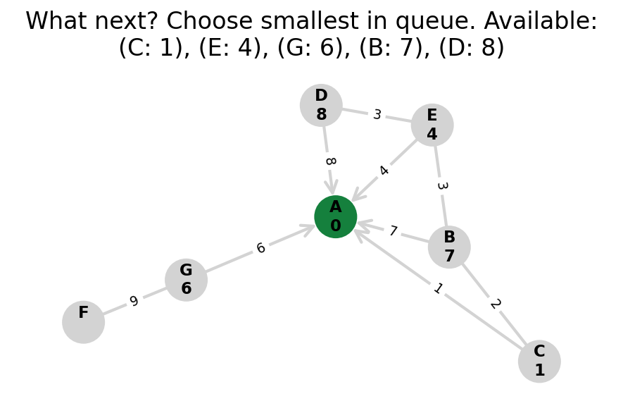
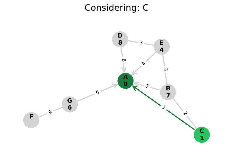
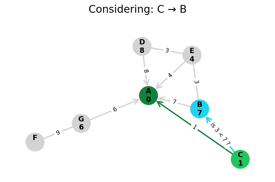
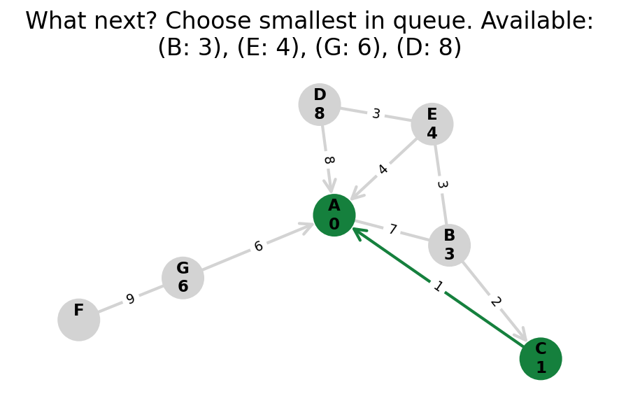
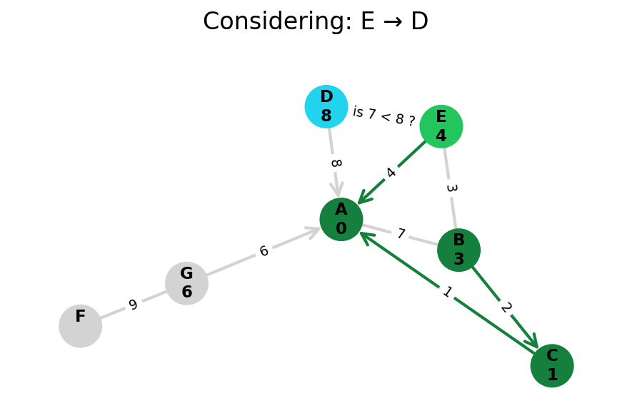
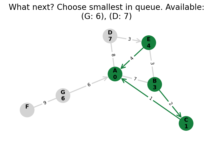
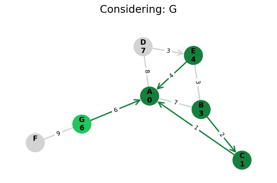
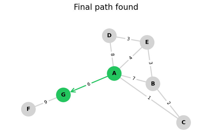
Dijkstra’s algorithm explores all nodes in the graph in increasing order of total distance from the start node.
It’s an instance of uniform cost search. It’s also a beautiful case of a greedy algorithm that finds optimal solutions.
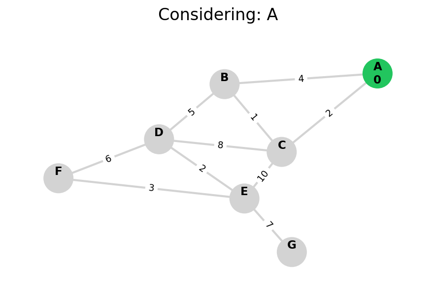
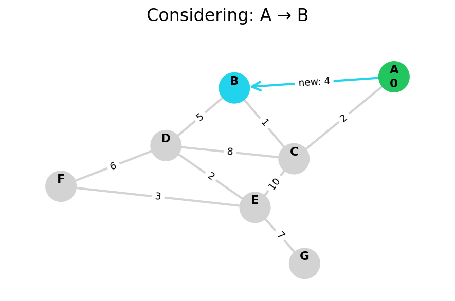
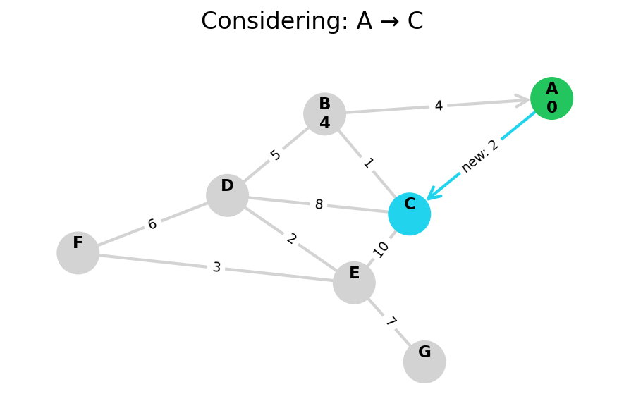
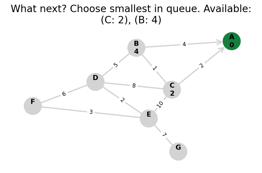
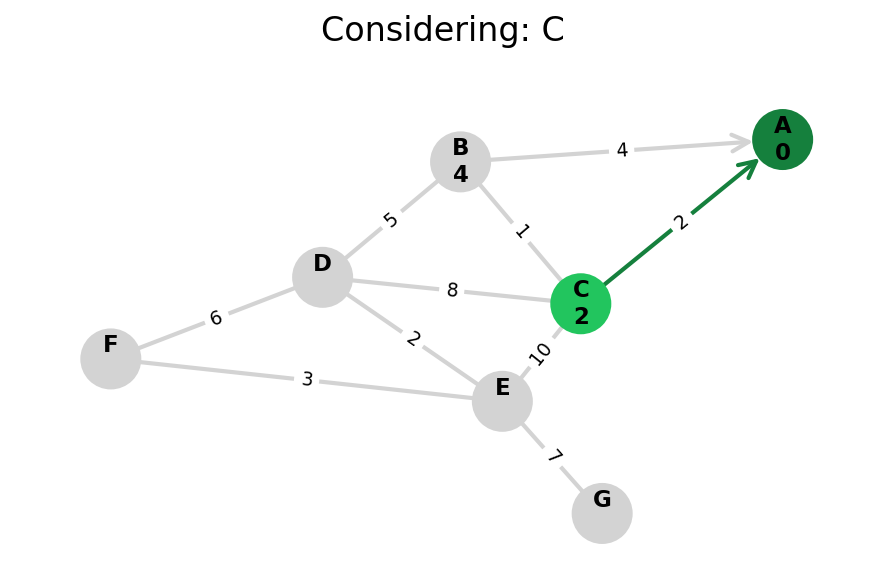
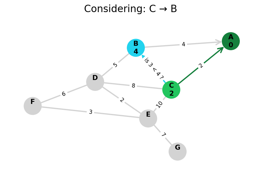
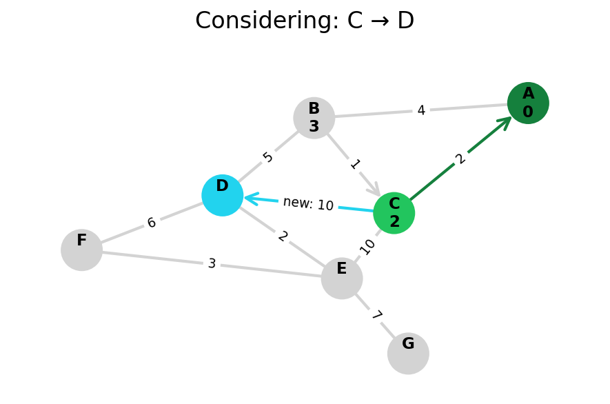
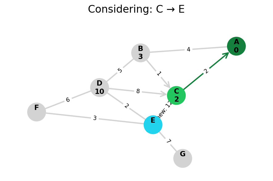
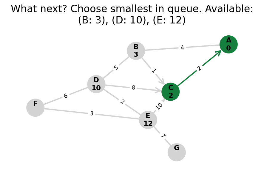
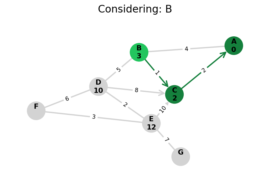
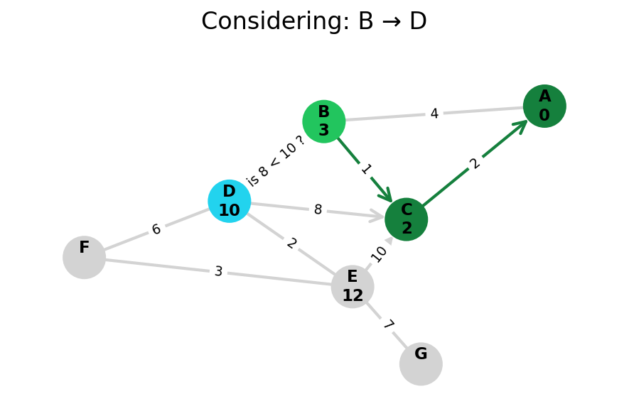
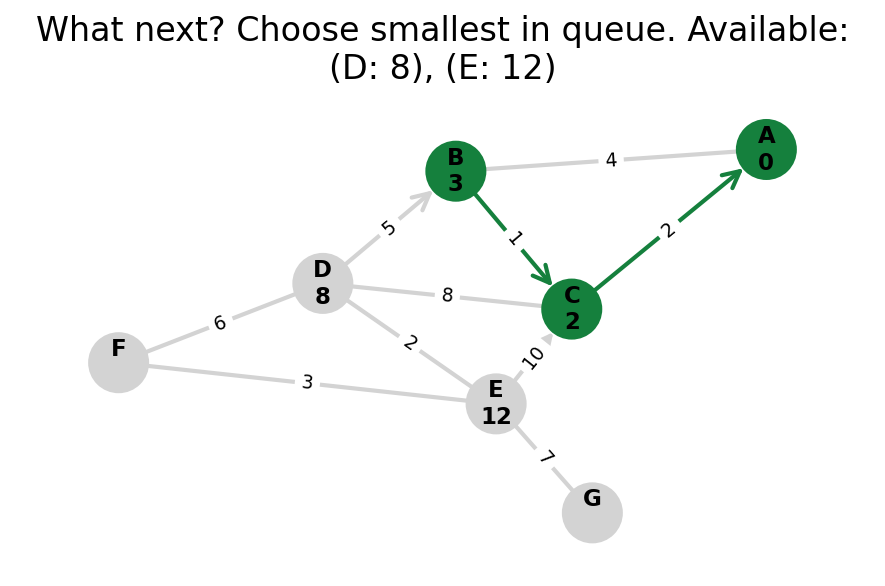
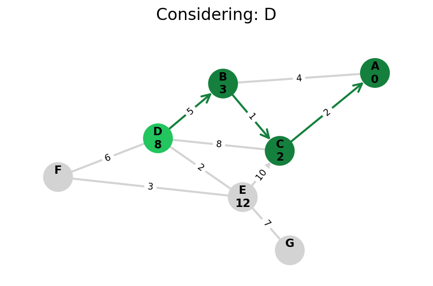
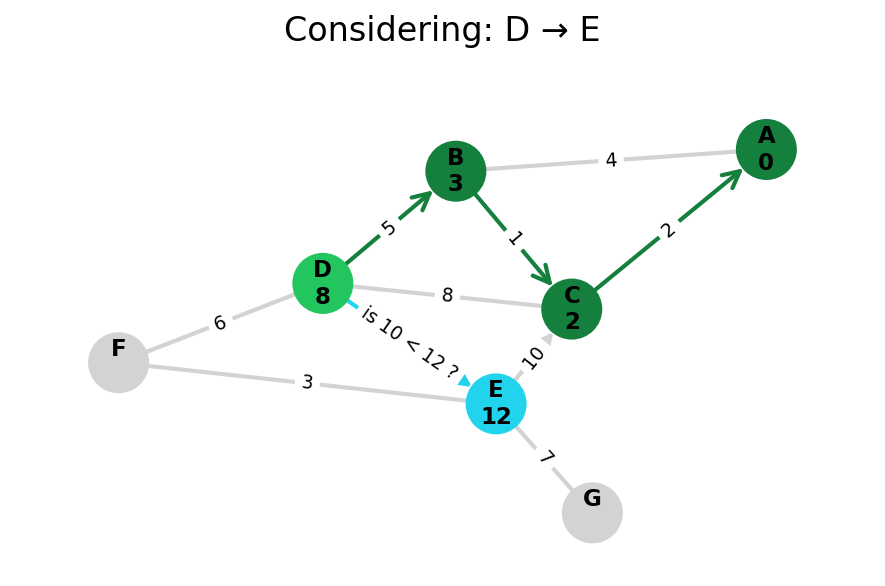
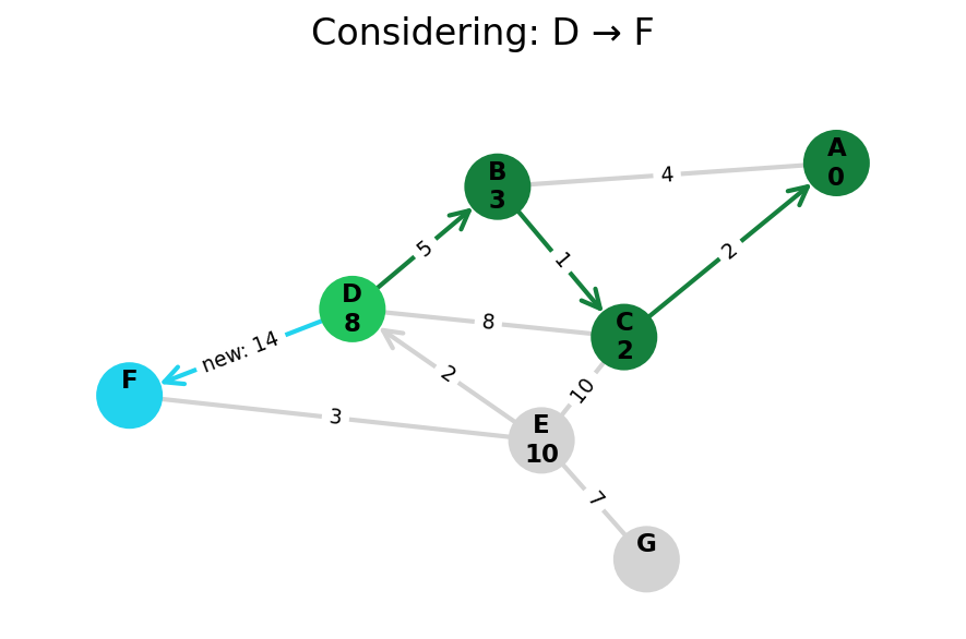
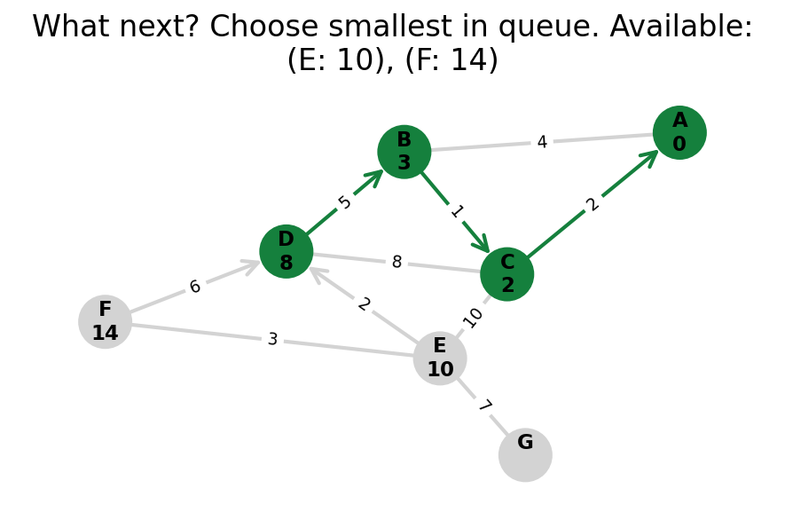
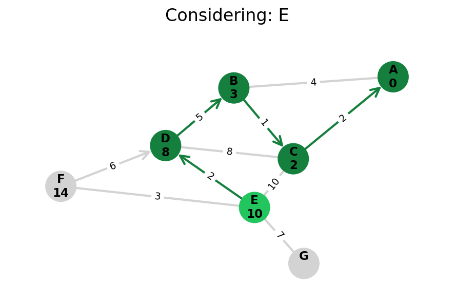
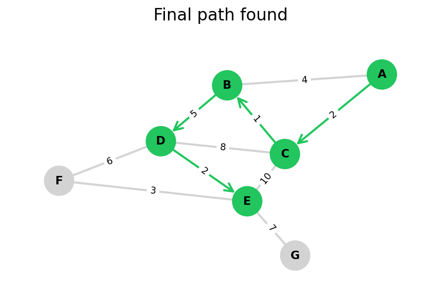
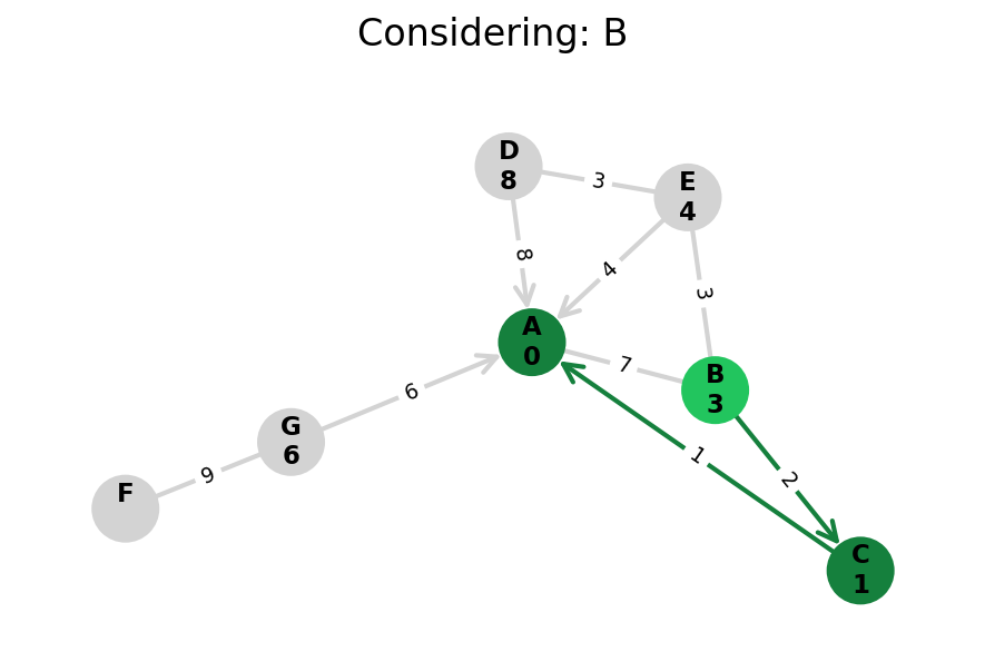
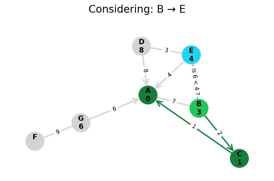
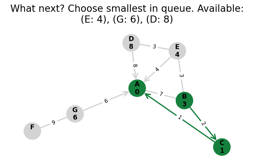
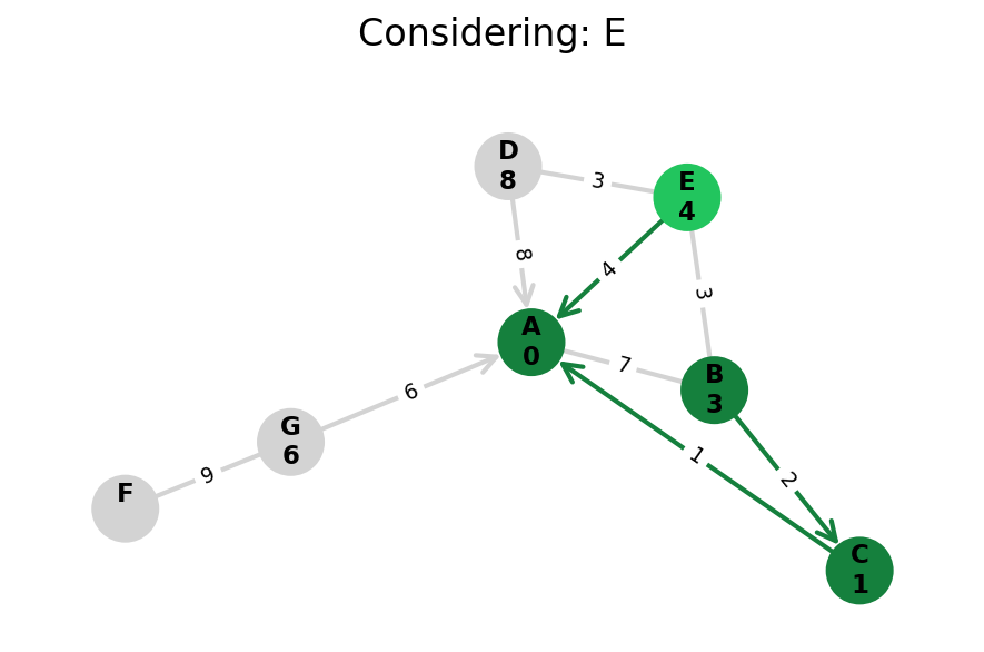
Here, I stop the algorithm once end is found. Use the controls below the image to the right to skip around and pause at your own pace.
Here’s a pseudocode implementation:
def dijkstra(graph: Graph[str], start: str):
    previous: dict[str, Optional[str]] = {start: None}
    heap = Heap([(start, 0)]).order_by(1)  # order by dist
    finished: set[str] = set()

    while len(heap) > 0:
        node, dist = heap.pop()
        finished.add(node)
        for neighbor, edge in graph[node].items():
            if neighbor in finished:
                continue
            neighbor_dist = dist + edge["weight"]
            if neighbor not in heap or neighbor_dist < heap.get(neighbor):
                previous[neighbor] = node
                heap.set(neighbor, neighbor_dist)

    return previous
A sketch of Dijkstra’s in pseudocode, finding the shortest path from start to all other nodes. Assume superpowered heap that supports get() by key and set() (which knows how to decrease()). Full implementation in the expandable snippet below.
Click to show a full Dijkstra's Algorithm in Python
class HeapNode:
    __slots__ = ["name", "dist"]

    def __init__(self, name: str, dist: float):
        self.name = name
        self.dist = dist

    def __lt__(self, other: "HeapNode"):
        """Only comparison required to support heap operations."""
        return self.dist < other.dist


def dijkstra(graph: nx.Graph[str], start: str, end: str):
    """Dijkstra's algo

    All you really need to know about nx.Graph is that
    graph[node].items() iterates over node's (neighbor, edge) tuples.
    """
    distances: dict[str, float] = {start: 0}
    previous: dict[str, Optional[str]] = {start: None}
    heap: list[HeapNode] = [HeapNode(start, 0)]
    finished: set[str] = set()
    while len(heap) > 0:
        heap_node = heapq.heappop(heap)
        node, dist = heap_node.name, heap_node.dist

        # allowing heap duplicates for lower costs (see note)
        if node in finished:
            continue
        assert dist == distances[node]
        finished.add(node)

        # optional: stop early once end found
        if node == end:
            break

        for neighbor, edge in graph[node].items():
            # we don't need to consider paths to neighbors if they're
            # already finished because we're guaranteed to already have
            # the shortest path to them.
            if neighbor in finished:
                continue
            weight = edge["weight"]
            neighbor_dist = dist + weight

            if (
                neighbor not in distances or
                neighbor_dist < distances[neighbor]
            ):
                distances[neighbor] = neighbor_dist
                previous[neighbor] = node
                heapq.heappush(heap, HeapNode(neighbor, neighbor_dist))

    return distances, previous
From my source repo. Finds the shortest path from start to end, stopping early, and accommodating that Python’s builtin heap doesn’t support lookup by key or decrementing a value (though the latter has an internal API). Actually, this is still an abstracted snippet, because I have graph visualization calls in the real version (to generate the images below), which take up more code than the algorithm itself.
Some notes on implementing Dijkstra’s algorithm:
-
Conceptually, two things helpful to remember:
-
All distances we save are implicitly distances from the start node, unless we’re dealing with an edge directly.
-
Once a node is properly visited because it was the lowest on the heap (i.e., not because it was distance-checked from a neighbor), then it is finished. I.e., the shortest path from
startto it has been found and will not change.
-
-
I think classically, you initialize data structures with all nodes — i.e., infinity distance, back pointers to null. I removed this because it seemed unnecessary.
-
The pseudocode implementation finds the shortest path from
startto all nodes. I think having a targetendnode is common, so I wrote my implementation to stop immediately when a path toendis found. -
A pure implementation, like the one I wrote in the pseudocode, only needs to remember unvisited nodes’ shortest distances from the start (
heap), back-links (previous) to be able to reconstruct the path, and which nodes arefinished. In practice, this would require a heap that supports access by key, as well as decrementing a key’s value (priority). Python’sheapqsupports neither, so we decouple it into:distances: a mapping from nodes to the shortest distance found so farheap: now saves every new shortest distance found to each node. I.e., a node may be entered into the heap many times. This ends up being fine (see next).finished: is now used not just to avoid adding to heap, but also to ignore when (a duplicate is) pulled off the heap.
-
New: A clever implementation can actually use
distancesto removefinished: only add toheapwhen a shorter distance is found, and ignore a node that’s popped off the heap if it’s worse than the current saved shortest distance. I keptfinishedin my code because I render finished nodes differently (dark green) in the visualization. -
Adding duplicates to the heap because it doesn’t support looking up and decreasing a key’s value is actually not so bad.
- Our case is simpler than the general case because we only add shorter distances. So, they’ll always come up first in the heap. So, we don’t need to worry about maintaining a separate map to mark old heap items as invalid. We just maintain the
finishedset and only process a node once. - In terms of complexity, we may add O(E) nodes to the heap rather than O(V). For space, as E <= V^2 in a graph, the memory footprint could be squared in a large enough graph. But for time, it’s not bad. Since (binary) heap operations are log(n), an operation on an E = V^2 sized heap is log(V^2) = 2log(V), which hits the same big-O as log(V) (operations on a V-sized heap).01
- Our case is simpler than the general case because we only add shorter distances. So, they’ll always come up first in the heap. So, we don’t need to worry about maintaining a separate map to mark old heap items as invalid. We just maintain the
Because Dijkstra’s expands in increasing order of distance, it may visit many nodes which don’t make progress towards its goal. We can see this happen in the example below.
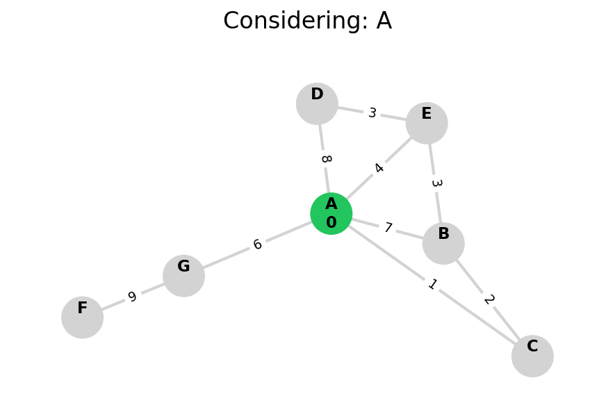
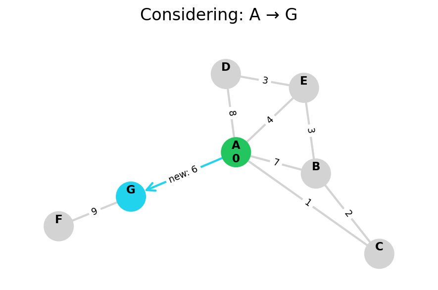
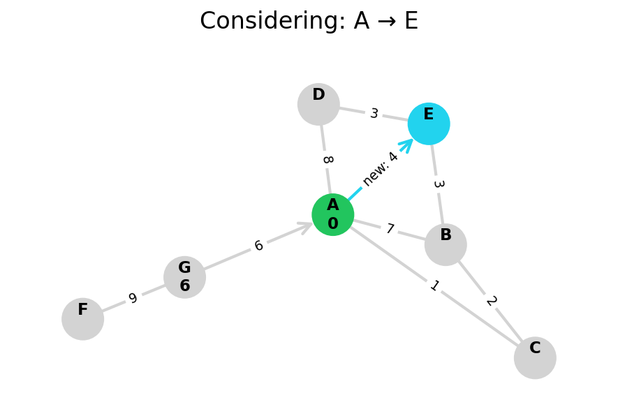
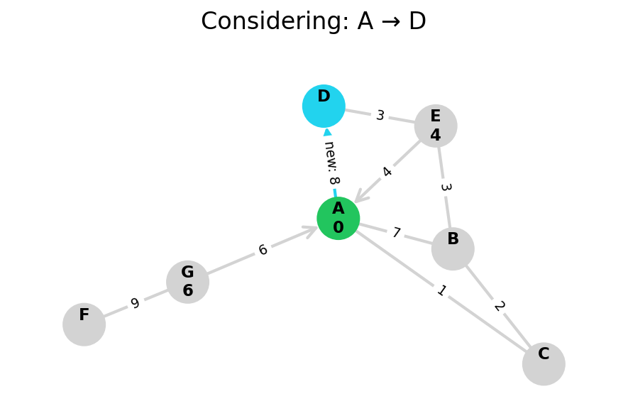
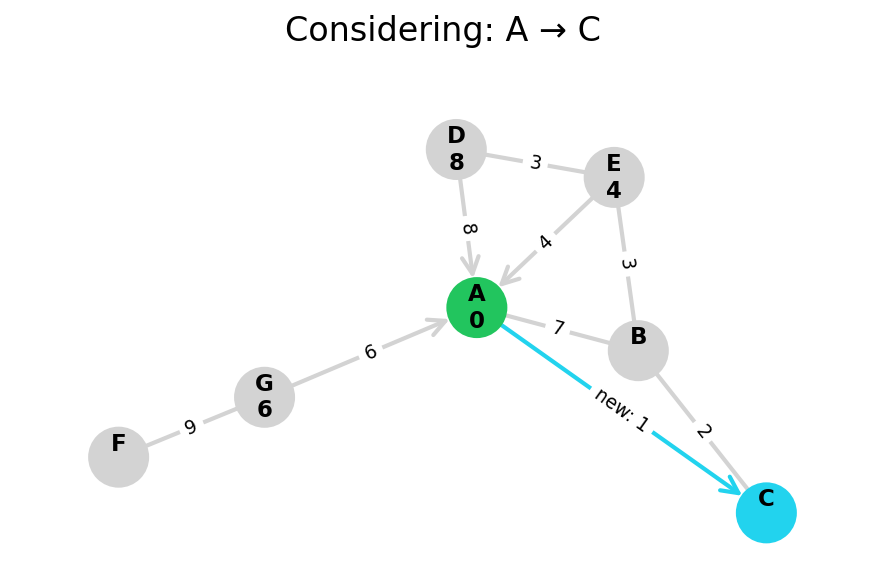
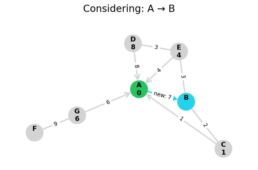
When a heuristic is available to judge whether we’d make progress towards our goal—like if we’re searching on a graph which also lives in Euclidean space—then we can upgrade Dijkstra’s to A*.
A*
A* search is Dijkstra’s, plus a heuristic h(n) that estimates the cost from a node n to the goal.
While Dijkstra’s technically doesn’t need a goal and can find the shortest path to all nodes, A* is goal-based because the heuristic incorporates distance-to-goal in the priority queue ordering.
Because we have a few distances now, we’ll use common notation:
- $g(n) \quad$ distance from start to $n$
- $h(n) \quad$ heuristic-estimated distance from $n$ to goal
- $f(n) = g(n) + h(n)$
def a_star(
    graph: Graph[str],
    start: str,
    goal: str,
    h: Callable[[str], float]
):
    previous: dict[str, Optional[str]] = {start: None}
    heap = Heap([(start, h(start), 0)]).order_by(1)
    #        ordered by f(n) ^     ^
    #         but we'll also use g(n)
    finished: set[str] = set()

    while len(heap) > 0:
        node, _, g_node = heap.pop()
        if node == goal:
            return previous
        finished.add(node)

        for neighbor, edge in graph[node].items():
            if neighbor in finished:
                continue
            g_neighbor = g_node + edge["weight"]
            f_neighbor = g_neighbor + h(neighbor)
            if (
                neighbor not in heap or
                f_neighbor < heap.get(neighbor)[1]
            ):
                previous[neighbor] = node
                heap.set((neighbor, f_neighbor, g_neighbor))

    return None  # goal not found!
A sketch of A* in pseudocode, finding the shortest path from start to goal. If our heuristic isn’t admissible or consistent, we’d want a more general-purpose implementation (e.g., re-opening finished nodes). As with the Dijkstra’s pseudocode, assumes superpowered heap with get() and set().
Some notes:
- multiple goals, can reach any? what about
min(h(g1), h(g2), ..., h(gn))? - we can think of
h(n) = 0as reducing to Dijkstra’s
An A* heuristic has two potential properties we care about: admissibility and consistency.
-
An admissible heuristic never overestimates the cost to the goal. It can underestimate—e.g., “bird flies” distance (L2) when you have to move on roads or through slower terrain. Admissibility is necessary for solutions found to be optimal.
- Example of overestimation leading to unoptimal solution: you travel to through
vto get tog.v'would have been faster, but its distance togwas overestimated, so it was explored later.
- Example of overestimation leading to unoptimal solution: you travel to through
-
A consistent (monotonic) heuristic requires estimates drop by at most the cost of moving. I.e., the triangle inequality. $h(a) \leq h(b) + \text{edge}(a, b)$. An inconsistent heuristic means we may need to “re-open” nodes as a faster path may be found.
- Example of inconsistency: picking from two heuristics (like indoor Manhattan vs outdoor Euclidean), estimates become inconsistent at the boundary.
Topological Sort
A topological ordering of a directed graph is a list of nodes such that any node $v$ comes after all of its dependencies. I.e., for every directed edge $u$→$v$, $u$ comes before $v$ in the ordering.
When can this be done? A topological ordering is possible on any directed graph without cycles (a DAG). Every DAG has at least one topological ordering, and one can be found in linear time.
Why would you do this? Job scheduling: computers (Airflow) or humans (project management). Spreadsheet cell update order. Makefiles.
Because I find the dependent vs dependency wording confusing, I’ll use parents and children here.
Kahn’s Algorithm
Kahn’s Algorithm is a topological sorting algorithm that runs in O(|V| + |E|).
The idea of Kahn’s algorithm is:
- start a worklist with nodes with no parents
- every time you visit a node in the worklist:
- add it to the result
- delete the edges from it to all its children
- if any child has no parents, add it to the worklist
Different worklist traversal orders (e.g., stack vs queue) can result in different topo orderings.
Implementation notes: By using an auxiliary data structure to quickly lookup a node’s (remaining) parents in O(1) time, we can also mutate this data structure and avoid mutating the underlying graph.
Click to show Kahn's Algorithm in Python
"""Kahn's algorithm to topologically sort a DAG.

Common graph representations:
- adjacency list: each node holds their set of edges (a has a->b, a->c)
- adjacency matrix: there's a VxV matrix where (a,b) has an entry for a->b
- incidence matrix: a VxE matrix, where an edge (a,b) has exactly two entries at a and b

NOTE: To avoid the mental overload of using "dependency" vs "dependant" correctly, I'm
going to abuse "child" and "parent" here.

Kahn's pseudocode:
- answer = []
- worklist = all nodes with no parents (incoming edges)
- while worklist isn't empty:
    - pop item a
    - add to answer
    - for all of a's children b in a->b:
        - remove the edge (a, b) from the graph
        - if b has no more parents (incoming edges), add it to worklist
- answer is a topo sort if the graph has no more edges (AKA len(answer) = |V|)
- otherwise, the graph has at least one cycle

Running time: O(|V| + |E|)
Space: O(|V|)
    - (all nodes will end up in answer; worklist OK as mutually exclusive w/ answer)
    - you don't actually need to mutate the graph if you're counting in-degree

Any worklist ordering is valid, because everything in the worklist has no parents. Thus,
stack vs queue vs random (vs ...) may give different answers.

Kahn's requires a few different graph operations:
1. find all nodes with no parents: O(|V|) is fine because outside of loop

But ideally we'd like to do the next two in O(1) time:
2. remove edge from graph
3. lookup whether node has any parents

2. is trivial in any representation (given the right references), but I think 3.
requires an O(|V|) or O(|E|) scan out of the box. We can track additional data to speed
up 3.
"""

from collections import defaultdict
from dataclasses import dataclass
from typing import Optional


@dataclass(slots=True)
class GraphNode:
    name: str
    children: list["GraphNode"]


def make_indegree_and_edges(graph: list[GraphNode]):
    in_degree: defaultdict[str, int] = defaultdict(lambda: 0)
    n_edges = 0
    for node in graph:
        in_degree[node.name] += 0  # just to ensure it's in the graph
        for child in node.children:
            in_degree[child.name] += 1
            n_edges += 1
    return in_degree, n_edges


def kahn(graph: list[GraphNode]) -> Optional[list[GraphNode]]:
    in_degree, n_edges = make_indegree_and_edges(graph)
    topo = []
    worklist = [node for node in graph if in_degree[node.name] == 0]
    while len(worklist) > 0:
        node = worklist.pop()  # or popleft() if deque
        topo.append(node)
        for child in node.children:
            n_edges -= 1
            in_degree[child.name] -= 1
            if in_degree[child.name] == 0:
                worklist.append(child)

    if n_edges == 0:
        return topo  # ordering
    else:
        return None  # graph had cycles


def make_example_graph():
    """
    c  a
    |  ↓
    |  b
    ↘ ↙
     d
    """
    d = GraphNode("d", [])
    b = GraphNode("b", [d])
    c = GraphNode("c", [d])
    a = GraphNode("a", [b])
    return [a, b, c, d]


def main() -> None:
    graph = make_example_graph()
    topo = kahn(graph)
    print("Found topo ordering:")
    if topo is None:
        print("None: graph had cycles")
    else:
        print(", ".join([n.name for n in topo]))


if __name__ == "__main__":
    main()
From my source repo.
Footnotes
Gemini also points out that Python’s
heapqhas a C implementation, whereas a custom Python-only data structure won’t. So the 2x factor will probably be dwarfed in practice by the implementation language. Of course, any actual usage that cares should measure. ↩︎