Ordinary least squares, ℓ² (ridge), and ℓ¹ (lasso) linear regressions

Preface #

I wrote this in 2017, and am posting it now in 2021. I was surprised how difficult it was to find complete information about linear regressions in one place: the derivations of the gradients, how they get their properties (e.g., lasso’s sparsity requiring coordinate descent), and some simple code to implement them. I tried to be careful about vector shapes and algebra, but there are probably still minor errors, which are of course my own.

One big goof I had was running this on MNIST, which ought to be treated as a classification problem per class (e.g., with logistic regression), rather than trying to regress each digit to a number (e.g., the digit “1” to the number 1, and the digit “5” to the number 5). I should have ran this code on a true regression dataset instead, where you do want real numbers (rather than class decisions) as output.

However, the silver lining is that after this goof, I was in a computer architecture class where we needed to run MNIST classification on FPGAs, and the starter code had made exactly this same mistake—they were doing linear instead of logistic regression! Making that simple switch resulted in such an accuracy boost that the classifier became one of the pareto optimal ones.

The repository for this project, which contains the full writeup below, as well as simple pytorch code to implement it, is here:

Enjoy!

– Max from 2021

Goal #

Build linear regression for MNIST from scratch using pytorch.

Data splits #

MNIST (csv version) has a 60k/10k train/test split.

I pulled the last 10k off of train for a val set.

My final splits are then 50k/10k/10k train/val/test.

Viewing an image #

Here’s an MNIST image:

Here it is expanded 10x:

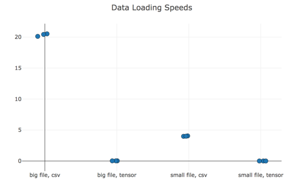
Data loading: CSV vs binary (“tensor”) #

y-axis is seconds taken to load the file; lower is better. Result: binary is way faster.

Naive regression to scalar #

In this we regress each image to a scalar that is the number represented in that image. For example, we regress the image to the number 5.

Disclaimer: this is a suboptimal approach. If you’re going to treat was is really a classification problem (like MNIST) as regression, you should regress to each class independently (i.e., do 10 regression problems at once instead of a single regression). Explaining why would take math that I would have to talk to people smarter than me to produce. I think the intuition is that you’re making the learning problem harder by forcing these distinct classes to exist as points in a 1D real space, when they really have no relation to each other. This is better treated as a logistic regression problem.

However: (a) if you’re confused like I was, you might try it, (b) if you’re bad at math like me, it’s simpler to start out with a “normal” regression than 10 of them, (c) I’m kind of treating this like a notebook, so might as well document the simple → complex progression of what I tried.

So here we go.

Notation #

Definitions:

Math reminders and my notation choices:

NB: While the derivative of a function f : ℝⁿ → ℝ is technically a row vector, people™ have decided that gradients of functions are column vectors, which is why I have transposes sprinkled below. (Thanks to Chris Xie for explaining this.)

Ordinary least squares (OLS) #

Loss (average per datum):

Using the average loss per datum is nice because it is invariant of the dataset (or (mini)batch) size, which will come into play when we do gradient descent. Expanding the loss function out for my noob math:

Taking the derivative of the loss function with respect to the weight vector:

We can set the gradient equal to 0 (the zero vector) and solve for the analytic solution (omitting second derivative check):

Doing a little bit of algebra to clean up the gradient, we’ll get our gradient for gradient descent:

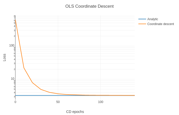
We can plot the loss as we take more gradient descent steps:

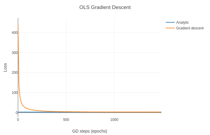
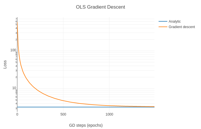
… but it’s hard to see what’s happening. That’s because the loss starts so high and the y-axis is on a linear scale. A log scale is marginally more informative:

To instead do coordinate descent, we optimize a single coordinate at a time, keeping all others fixed. We take the derivative of the loss function with respect to a single weight:

Setting the derivative equal to zero, we can solve for the optimal value for that single weight:

However, this is an expensive update to a single weight. We can speed this up. If we define the residual,

then we can rewrite the inner term above as,

and, using (t) and (t+1) to clarify old and new values for the weight, rewrite the single weight optimum as:

After updating that weight, r is immediately stale, so we must update it as well:

We can compute an initial r and we can precompute all of the column norms (the denominator) because they do not change. That means that each weight update involves just the n-dimensional vector dot product (the numerator) and updating r (n-dimensional operations). Because of this, one full round of coordinate descent (updating all weight coordinates once) is said to have the same update time complexity as one step of gradient descent (O(nd)).

However, I found that in practice, one step of (vanilla) gradient descent is much faster. I think this is because my implementation of coordinate descent requires moving values to and from the GPU (for bookkeeping old values), whereas gradient descent can run entirely on the GPU. I’m not sure if I can remedy this. With that said, coordinate descent converges with 10x fewer iterations.

But how well do we do in regressing to a scalar with OLS?

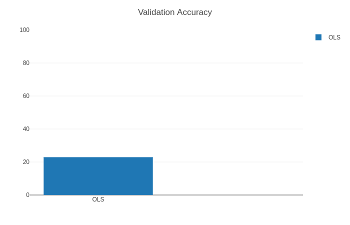
Not very well.

Ridge regression (RR) #

Loss:

NB: For all regularization methods (e.g., ridge and lasso), we shouldn’t be regularizing the weight corresponding to the bias term (I added as an extra feature column of 1s). You can remedy this by either (a) centering the ys and omitting the bias term, or (b) removing the regularization of the bias weight in the loss and gradient. I tried doing (b) but I think I failed (GD wasn’t getting nearly close enough to analytic loss), so I’ve left the normalization in there for now (!).

Derivative:

(Being a bit more liberal with my hand waving of vector and matrix derivatives than above)

Analytic:

NB: I think some solutions combine n into λ because it looks cleaner. In order to get the analytic solution and gradient (descent) to reach the same solution, I needed to be consistent with how I applied n, so I’ve left it in for completeness.

Gradient:

(Just massaging the derivative we found a bit more.)

Coordinate descent:

The derivative of the regularization term with respect to a single weight is:

with that in mind, the derivative of the loss function with respect to a single weight is:

In setting this equal to 0 and solving, I’m going to do some serious hand waving about “previous” versus “next” values of the weight. (I discovered what seems (empirically) to be the correct form by modifying late equations of the Lasso coordinate descent update, but I’m not sure the correct way to do the derivation here.) We’ll also make use of the residual .

As above, we update the residual after each weight update:

Lasso #

Loss:

Derivative:

Focusing on the final term, we’ll use the subgradient, and pick 0 (valid in [-1, 1]) for the nondifferentiable point. This means we can use sgn(x) as the “derivative” of |x|.

Substitute in to get the final term for the (sub)gradient:

NB: There’s no soft thresholding (sparsity-encouraging) property of LASSO when you use gradient descent. You need something like coordinate descent to get that. Speaking of which…

Coordinate descent:

setting this = 0, and again using the residual , we have:

NB: I think that here (and below) we might really be saying that 0 is in the set of subgradients, rather than that it equals zero.

There’s a lot going on. Let’s define two variables to clean up our equation:

From this, we can more clearly see the solution to this 1D problem:

This solution is exactly the soft threshold operator:

Rewriting this into its full form:

As with coordinate descent above, we need to update the residual r after each weight update (skipping the derivation; same as above for OLS):

Links #

• Table of regularized least squares functions (Wikipedia)
• The Matrix Cookbook (Petersen & Pedersen)
• OLS with matrices notes (possibly Rosenfeld?)
• Coordinate Descent (Gordon & Tibshirani)
• A Coordinate Descent Algorithm for the Lasso Problem (Chi)
• Deriving the lasso coordinate descent update (Fox)

Acknowledgements #

Many thanks to Chris Xie and John Thickstun for helping me out with math. All errors are my own.