Procedural City Layout Generation with GANs
Preface
This was my project for a computer graphics class I took back in 2017. (I’m writing this now in 2021.) I was interested in doing procedural city generation, but using machine learning to do it. As far as I could tell, that hadn’t been done before.
I was originally excited to do something like “grammar induction:” learning a grammar for how to generate cities based on looking at them. Grammar induction is a thing in natural language processing (NLP, my home field), but I didn’t really know anything about it.
In the end—as inevitably seems to happen with class projects—I ran out of time and did something simple: I trained a generative adversarial network (GAN) on image pairs to teach it how to add buildings to a map with other geographic features (stuff like roads, parks, and water). This still ended up being pretty cool.
If you interested, my code is available here:

Enjoy!
– Max from 2021
Table of Contents
Introduction
Motivation
Procedural generation affords the creation of large, authentic looking environments with far less time and effort than manual modeling.
The domain of urban procedural generation can be roughly split into three sub-problems: layout modelling (maps and roads), building modelling (3D geometries), and facade modelling (3D facades and textures).01 Exciting advances in all of these areas have led to remarkably realistic results, such as generating cities that expand over time02 and villages that grow based on their geography.03
While procedural generation offers great gains compared to manually creating content, a key problem still exists: the designers of such generation systems create the algorithms by manually designing and encoding grammars that produce realistic looking results. This process requires substantial domain expertise and significant trial and error. In other words, procedural generation does not remove the manual effort required to generate large cities; it simply shifts the effort from 3D modeling to algorithm design!
However, for city layouts, freely available data from crowdsourced map projects now exist. From this data, it may be possible to train a machine learning model that can automatically generate city layouts without any hand-tuned grammar rules.
In addition to simply removing the manual work of designing generation algorithms, a machine learning model offers other pragmatic advantages to virtual city creators. For example, a model would learn to generate cities in the style of the geographic area on which it was trained. An old European town will present different layout patterns than a bustling metropolis like Tokyo. A machine learning model could capture these differences simply by being retrained on different data, without needed to re-design the parameters or grammars of the generation algorithm.
Task
In this project, we approach the first domain of urban procedural generation: generating the layout for a city. Within this domain, we further restrict our focus to the following task: given a road network and city features (like water and parks), fill in the buildings inside of blocks. Figure 1 shows a visual depiction of our task.
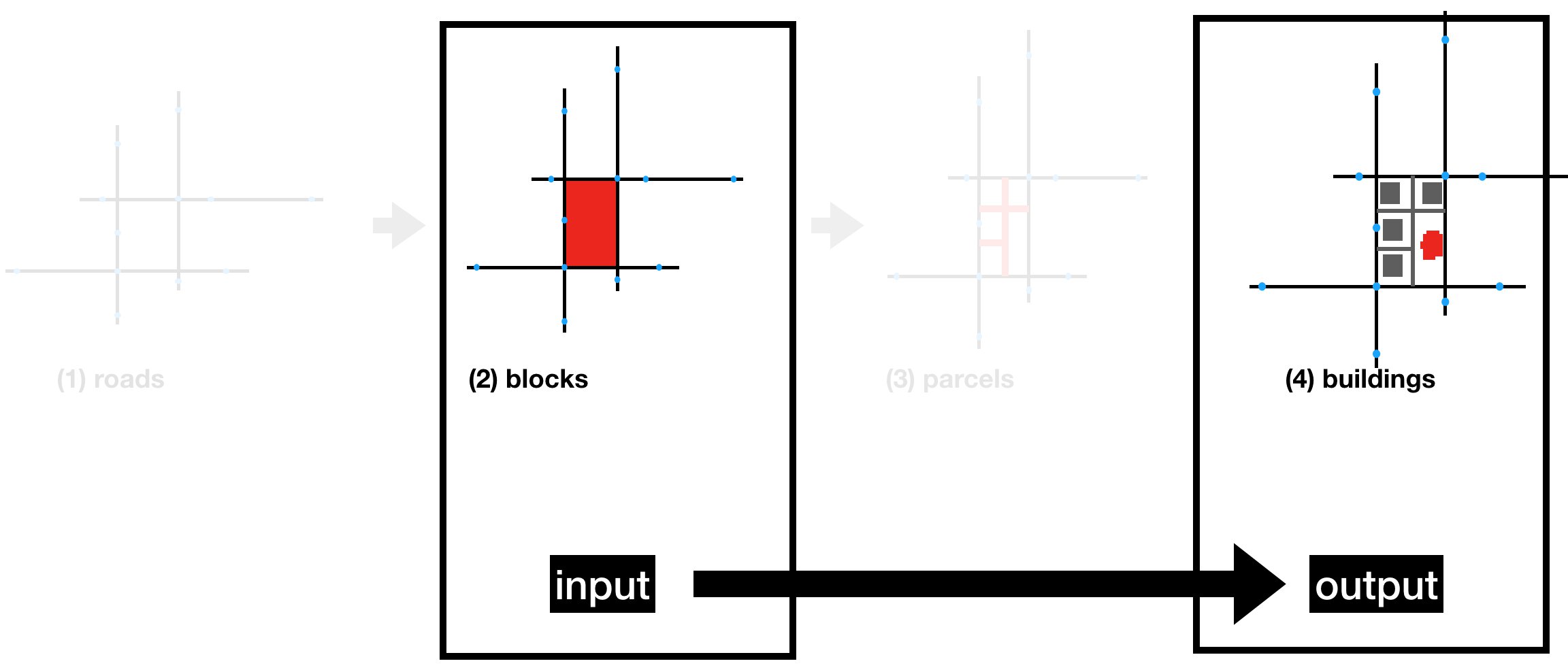
Figure 1: Task overview: given a road network, we attempt to directly fill in blocks with buildings.
We split this overall task into two subtasks. In the first subtask, we extract individual blocks with their buildings laid out on top of them. The goal is to generate the buildings for a single block at a time (Figure 2, upper half). This problem is more constrained, and provides an early test of the model’s capabilities.
In the second subtask, we provide a larger chunk of a city as input, and ask the model to fill in buildings in all the empty blocks provided (Figure 2, lower half). This task is more difficult, because more buildings must be generated and placed within the bounds of blocks. But because we also provide geographic features like water and parks in the input, a model can potentially take advantage of these semantic cues to generate layouts that are sensitive to their surroundings.
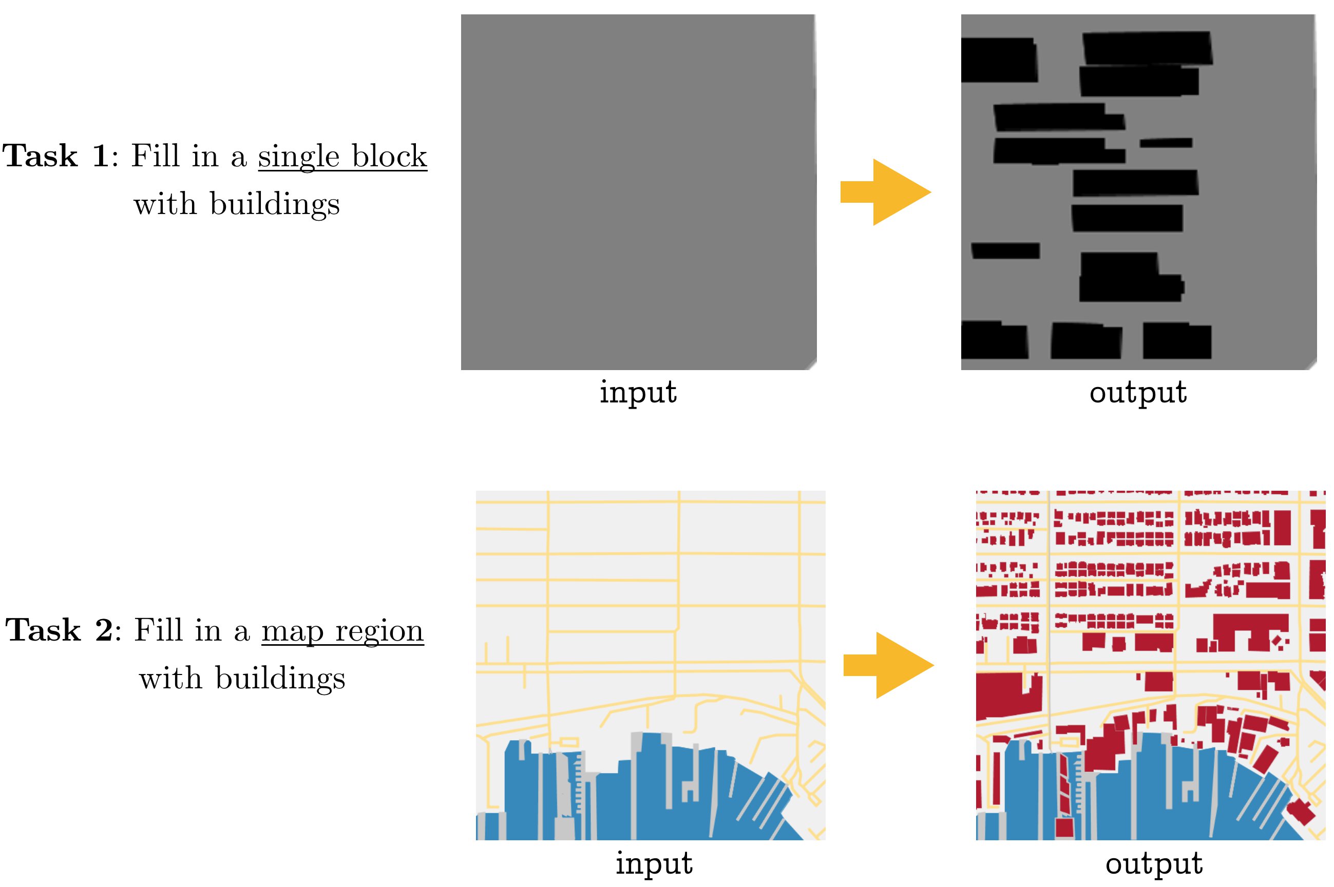
Figure 2: The two tasks we consider. In both cases, buildings must be generated on top of an input image. The difference is in the size of the region and the amount of geographic context provided.
Related Work
Inverse Procedural Modeling and Shape Learning
The idea of attempting to learn the parameters of a procedural generation model is called inverse procedural modeling. Though this has never been applied to city layout generation, it has been explored by several authors in other domains.
Wu et al. (2014) learn a split grammar for facades, preferring shorter descriptions as better representations of the grammar.04 Though it does not appear to use machine learning, Inverse Procedural Modeling by Automatic Generation of L-Systems (2010) propose an approach for reverse-engineering the parameters for an L-system (grammar) given input (in their case, 2D vector images) that was generated from one.05
Other authors have used graphical models to learn how to generate shapes and textures. Fan and Wonka (2016) learned a garphical model to generate 3D buildings and facades.06 Martinovic and Gool (2013) learn a 2D context-free grammar (CFG) from a set of labeled facades.07 In A Probabilistic Model for Component-Based Shape Synthesis (2012), the authors learn a graphical model trained on hand-modeled 3D shapes (like a dinosaur or a chair) in order to generate their own novel meshes.08 Toshev et al. (2010) take inspiration from classical natural language processing, and learn the parameters of a parsing model to map point clouds that represent roofs to a hierarchy of the roof’s components (e.g., main roof, hood over window, shed roof, etc.).09
City Modeling
Though these works do not use machine learning or inverse procedural generation, it is worth briefly touching upon city generation literature. Several papers present tools for editing or expanding a set of aerial images of cities. Aliaga et al. (2008, a) present a tool for making edits to an urban layout and generate roads and parcels to fit into the edited regions.10 In a followup work, Aglia et al. (2008, b) demonstrate another tool that, given an example image, synthesizes a new street network, and pastes in segments of the input image that fit well with the new road network.11
Other work focuses on generating cities from scratch. Weber et al. (2009) simulate a city’s growth over time, taking into account population growth and the according land use evolution.02:1 In Procedural Generation of Parcels in Urban Modeling (2012), the authors develop an algorithm for automatically splitting blocks (the spaces carved out by road networks) into parcels (areas of land ownership).12 Finally, Nishida et al. (2016) present a tool for editing road networks that takes into account the style and layout of example data.13
Dataset Creation
To the best of our knowledge, no previous work attempt the task of generating city layouts using machine learning. Because of this, a significant portion of the project time was spent collecting and preprocessing the data. For that reason, this section of the report gives a brief overview of this process.
Task 1: Individual Blocks
The first task we address is: given a block, generate the buildings on the block. For this task, we process maps data from OpenStreetMaps in order to identify and extract blocks.
Overview
The overall processes of the block extraction is shown below in Figure 3.
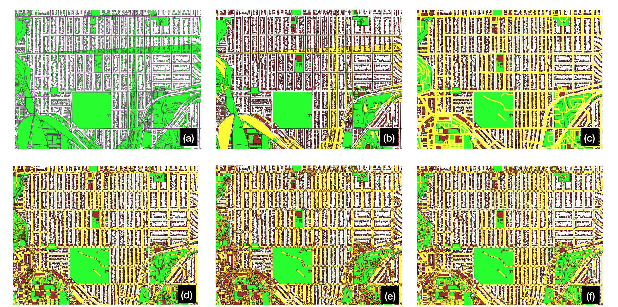
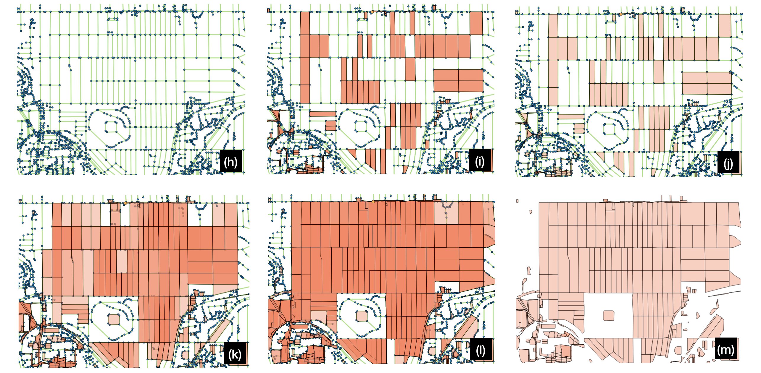
Figure 3: Stages of block extraction, done for the first task. The individual steps are described in the running text.
Block extraction broadly involved the following stages, each of which are illustrated above (Figure 3):
-
(a) OpenStreetMaps data is parsed from its native XML format, and all ways (collections of nodes) are rendered as polygons.
-
(b) Crowdsourced labels are aggregated into high-level features (such as buildings and roads) and polygons are colored according to their predominant feature.
-
(c) Roads are the only ways that should not be rendered as polygons; they are properly drawn as polylines.
-
(d) Nodes that serve as the underlying points for road ways are rendered.
-
(e) Road nodes are rendered in varying sizes to confirm that roads are drawn independently (i.e., informing us that intersections must be discovered).
-
(f) Nodes are recursively collapsed by finding nodes within a geographic euclidean distance and recursively building a map of backpointers.
-
(g) Now that nodes connect roads together, the map may be rendered as a graph, here shown in green and blue.
-
(i) First stage of block discovery: blocks of small distance (up to four edges) are discovered, but duplicates exist because the same block may be discovered by multiple nodes.
-
(j) Deduplication of identical blocks by keeping only unique sets of vertices. (Blocks are rendered with semi-transparency; the difference can be seen here from the last step because the blocks are a lighter shade of pink, indicating they only exist once.)
-
(k) Increasing the maximum search depth of the block discovery algorithm, we begin to find larger sets of nodes that encompass multiple blocks (darker pink regions). Because some blocks are defined by a large number of nodes due to having curvy roads, some are still missed.
-
(l) Further increasing the maximum block search depth, we recover all feasible blocks. At this point, heavy duplicate coverage plagues blocks due to the algorithm discovering many false enclosing blocks.
-
(m) Removal of false enclosing blocks. This is done by rendering all candidate blocks and removing any large candidates that fully enclose smaller candidates.
Graph Ring Discovery
A crucial part of the above process was devising an algorithm to find rings in the graph in order to identify candidate blocks. The algorithm is presented below in Python-like pseudocode with types. It is an augmented breadth-first search which tracks unique paths to vertices from paths starting at all neighbors of a start vertex.
NB: While presenting this algorithm, I was pointed to a simpler algorithm that takes into account the the geometry of the map: for each edge, follow edges of a maximum angle (e.g., clockwise) until the starting vertex is reached. For completeness, I still present here the algorithm that I devised to find rings in a graph.
# The overall algorithm searches from each vertex and returns the unique
# set of rings discovered.
def find_rings(graph: Dict[int, Set[int]]) -> List[List[int]]:
    return unique(find_rings_at(graph, n) for n in graph.keys())


# The bulk of the algorithm finds all rings that involve a chosen vertex up
# to a maximum depth.
def find_rings_at(graph: Dict[int, Set[int]], start: int,
                    maxdepth: int) -> List[List[int]]:
    # Setup.
    start_path = [start]  # type: List[int]
    shortest = {}  # type: Dict[int, List[List[int]]]
    q = Queue([(start, start_path)])

    # First, find sets of unique paths to surrounding vertices.
    while len(q) > 0:
        # Consider the vertex just found, a candidate "shortest path."
        cur, curpath = q.pop()
        if can_add_to_shortest(cur, curpath, shortest):
            if cur not in shortest:
                shortest[cur] = []
            shortest[cur].append(curpath)

        # Add neighbors to queue if we haven't explored to max depth yet.
        if len(curpath) < maxdepth:
            for neighbor in graph[cur]:
                # No backtracking per path.
                if neighbor not in curpath:
                    q.append((neighbor, curpath + [neighbor]))

    # Now, extract rings. They are discovered vertices with multiple paths.
    rings = []
    for candidate in shortest.keys():
        paths = shortest[candidate]
        if len(paths) > 1:
            # Use the first two paths found, and remove duplicate nodes
            # (first and last) from the second.
            p1 = paths[0]
            p2 = paths[1]
            rings.append(p1 + list(reversed(p2[1:-1])))

    return rings

# This helper algorithm determines whether a candidate path should be added
# to the set of shortest paths to a vertex.
def can_add_to_shortest(cur: int, curpath: List[int],
                        shortest: Dict[int, List[List[int]]]) -> bool:
    # If shortest hasn't found cur yet, then found a new shortest path.
    if cur not in shortest:
        return True

    # Crowdsourced map data; might have multiple edges between two vertices.
    if len(curpath) == 2:
        return False

    # Interesting case: We want to add only if we've found a new path to
    # this node that is unique; i.e., the middle nodes (excluding start and
    # cur) have nothing in common with any other paths.
    middle = set(curpath[1:-1])
    for p in shortest[cur]:
        exist_middle = set(p[1:-1])
        if len(exist_middle.intersection(middle)) > 0:
            return False
    return True
Algorithm 1: Ring discovery in a graph.
Block-Building Matching and Rendering
After discovering blocks, we then match each block to the set of buildings that lie on top of that block. To do this, we perform a point-in-polygon test for every vertex of every building onto the polygon defined by every block. While this test is an approximation of a polygon-in-polygon test, it works well in practice given the shape of blocks and buildings (there are no extreme, sharp concavities in the blocks).
Finally, we pick a standard resolution, and transform all blocks and the buildings on top of them to that fixed resolution output. We then use Processing14 to render all of the blocks in bulk, creating pairs of (empty, populated) blocks, rendering blocks in grey and buildings in black. Several example blocks are shown below in Figure 4.
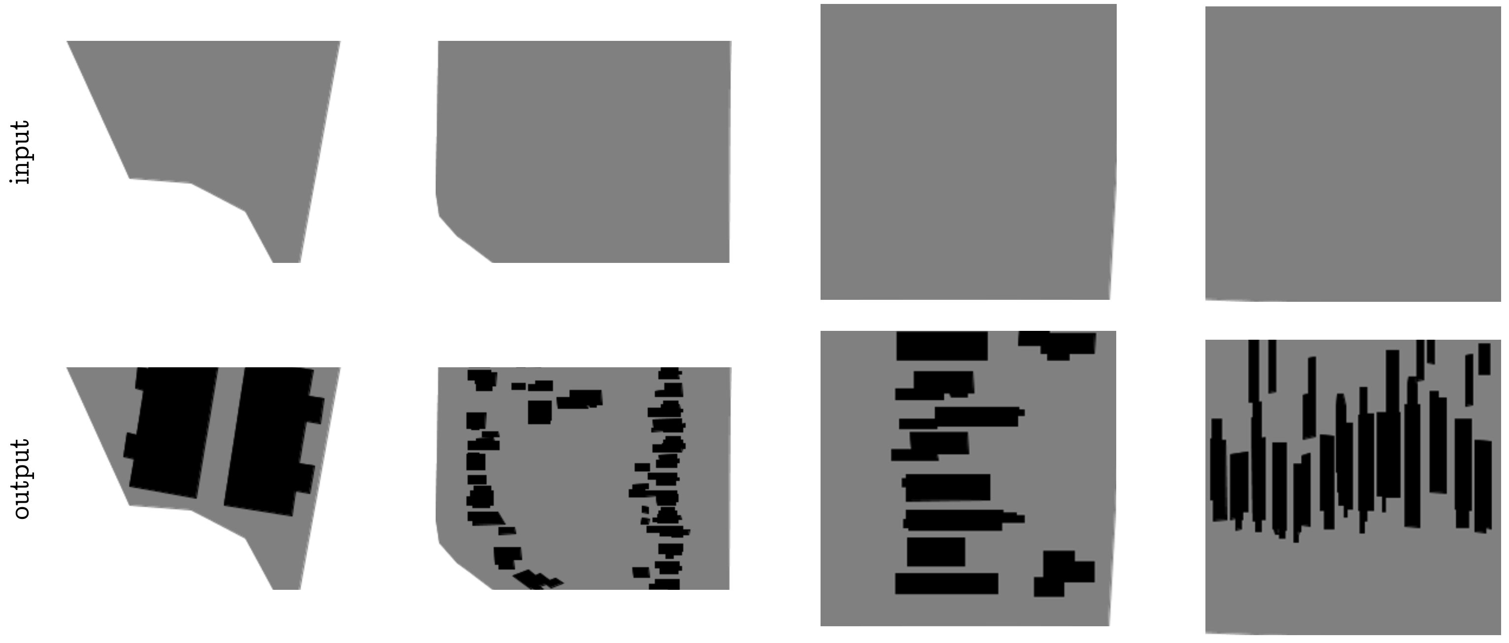
Figure 4: Four examples from the dataset for task 1: generating buildings for a block. Whereas some blocks have distinct shapes around which buildings must be placed (columns one and two), others provide almost no input but require specific outputs (columns three and four). Currently, uniform scaling per block results in a distorted appearance; this effect could be reversed in postprocessing, or future approaches could clip blocks to geographic bounds rather than scaling to a set pixel size.
We scrape five different regions of Seattle and extract all blocks with at least one building on them, giving a total of 1100 images, which we partition into train (521) / val (415) / test (164) splits such that the geographic regions do not overlap between the splits.
Task 2: Map Regions
The second task we address is: given a region of a map without any buildings, generate all of the buildings.
This task is simpler from a dataset creation perspective, because it simply involves rendering two versions of a map: one with most geographic features rendered except buildings, and the second including buildings as well.
Rendering Regions
The main challenge in creating a more realistic region-filling dataset is accurately rendering a broader range of geographic features. Recall in the dataset for task 1 that we render only block outlines and buildings. For task 2, we can encode more context and render additional geographic features, such as walkways, parks, and water. The difficulty in doing so is that these features are encoded with varying consistency, and at varying levels of abstraction.
Here are a few examples to illustrate how some features are labeled in the OpenStreetMap data:
| Tag(s) | Actual Geographic Feature |
|---|---|
| highway: yes | highway |
| highway: path | pedestrian walkway |
| man_made: pier, source: Yahoo! | walking area |
| source: Yahoo! | water |
| water: yes | water |
After selecting a variety of regions and manually adding mappings between tags, we end up with seven possible semantic categories per map that we render: (1) nothing (light grey) (blocks are colored this way), (2) buildings (red polygons), (3) roads (yellow lines), (4) water (blue polygons), (5) pedestrian areas (darker grey polygons), (6) pedestrian walkways (darker grey lines), (7) parks (green polygons). Four example renderings are shown below in Figure 5:
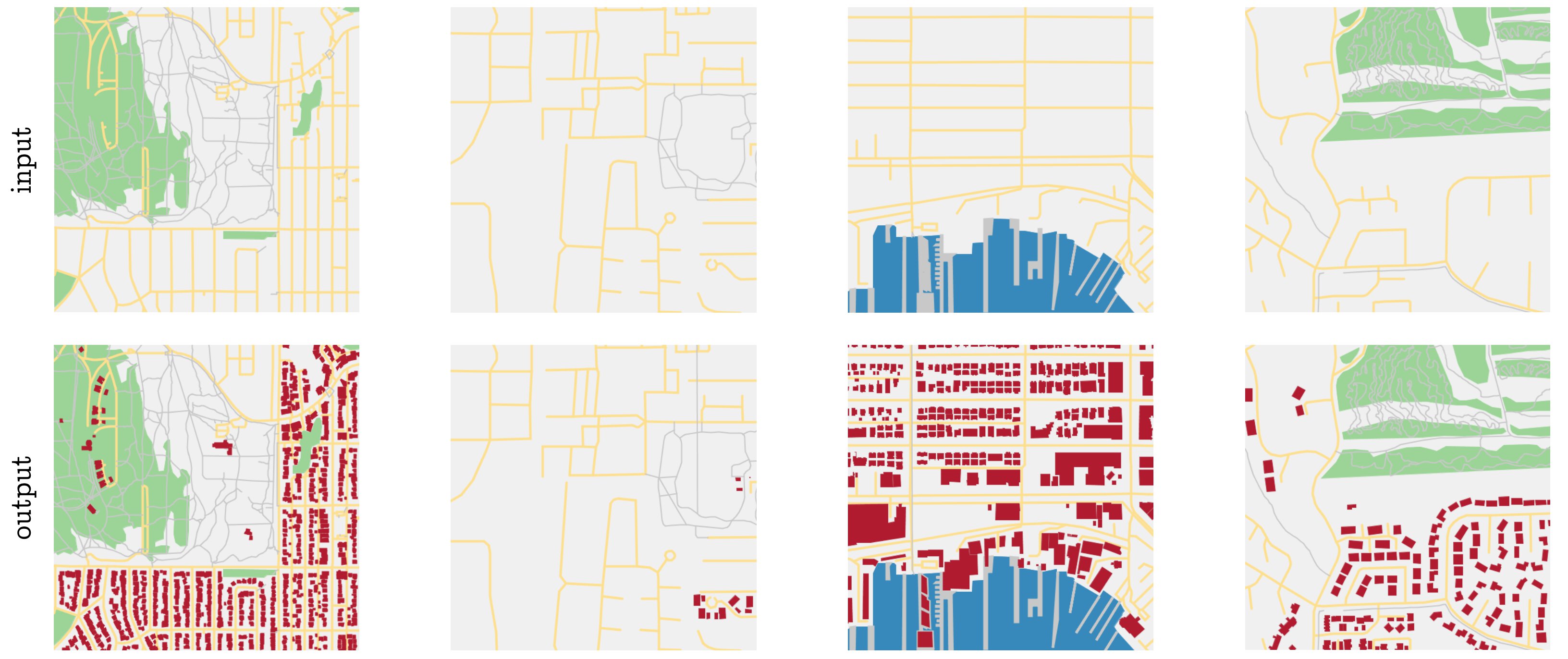
Figure 5: Four example regions in the dataset for task 2. The dataset exhibits a wide variety in the correct number of buildings in the output, as can be seen by the second column, which should be left mostly blank. Furthermore, note the presence of pedestrian footpaths around which buildings should not be generated (left and rightmost columns), the presence of buildings along the pier (third column), and the variety of block shapes around which buildings must be placed (columns one versus four).
Scraping
The only additional complication with rendering larger map segments is that the amount of map data required is significantly greater. We address this by building a small scraping pipeline that walks a given latitude, longitude geographic region by fixed window sizes (chosen to render well onto a square image).
We scrape a region encompassing the greater Seattle area: from the Puget Sound (W) to Sammamish (E), and from SeaTac (S) to Mountlake Terrace (N). This results in 2967 individual regions, which we filter to include only those with at least one building. After filtering, 1880 regions remain, which we partition into train (1680) / val (100) / test (100) splits.
Model
We use the conditional adversarial network, proposed by Isola et al. (2017).15
This model trains two networks, a generator, and a discriminator. The generator produces candidate output images, and the discriminator attempts to decide whether a given (input, output) pair is real, or whether the output was in fact created by the generator. They are trained together so that as the generator produces more realistic images, the discriminator also gets better at distinguishing them.
We use the same model presented in the paper by Isola et al., in which many more details can be found. We briefly note here that GAN (generative adversarial network) variants are notoriously difficult to train for two reasons. The first is that they require a careful balance between the generator and discriminator; if the discriminator is too effective, the generator can never fool it, and receives no training signal, while the reverse is true if the discriminator is easily tricked. The second is the problem of “mode collapse,” which happens when the generator finds a single output that the discriminator believes, and simply produces that identical output continuously. The second issue is less prevalent in conditional GANs, because the discriminator also receives the input; however, in our particular dataset, many inputs look identical, especially for the first task (there are many uniform grey squares as input).
Experimental Results and Discussion
Task 1
At the beginning of training, the model has trouble producing coherent shapes, and has not yet learned that it should only output one of three color values. This can be seen in Figure 6 with the multicolor banding on the right side of the image. However, it is able to immediately learn to reproduce the grey outline of the input block, and never draws black (buildings) on top of white (empty space).
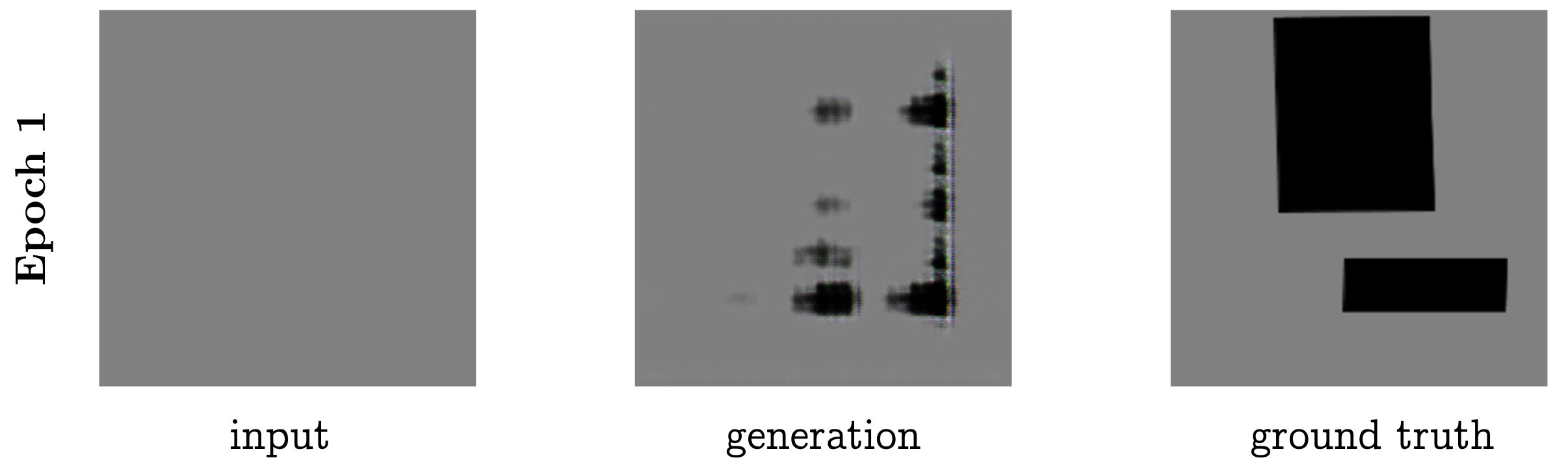
Figure 6: Task 1, after 1 epoch (pass over training data).
After nine epochs, the model is able to produce more ambitious shapes (Figure 7), but the shapes are too densely connected and rounded to be convincing enough to fool a human judge.
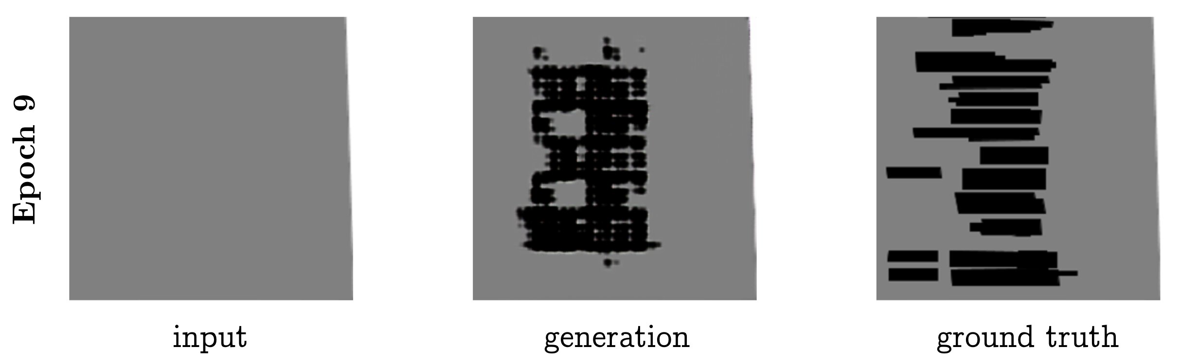
Figure 7: Task 1, after 9 epochs.
By the the end of training, the model is able to generate fairly convincing filled-in blocks. It is interesting to note that the L1 loss does not drop after about ten epochs, but the visual quality continues to improve. This can be understood by looking at one of the final outputs, in Figure 8. Without the gold output (far right), it would be difficult to tell whether the generation (middle) is correct. In that sense, it may well fool a discriminator, human or neural network. However, the L1 distance from the generated image to the gold is terrible, as it got the buildings almost completely wrong.
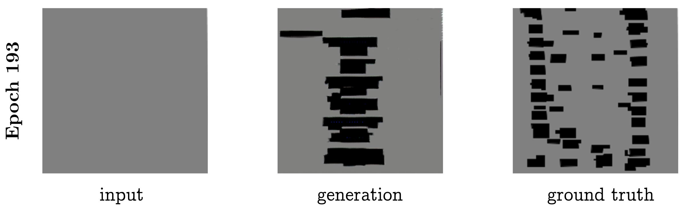
Figure 8: Task 1, after 193 epochs. (The model was trained for 200 epochs in total.)
Mode collapse
One question we were interested to investigate is: does the conditional adversarial network suffer from mode collapse in this task?
During the middle of training, we observed what appeared to be mode collapse, as can be seen in Figure 9. The model repeatedly generates a single building near the bottom of the image.
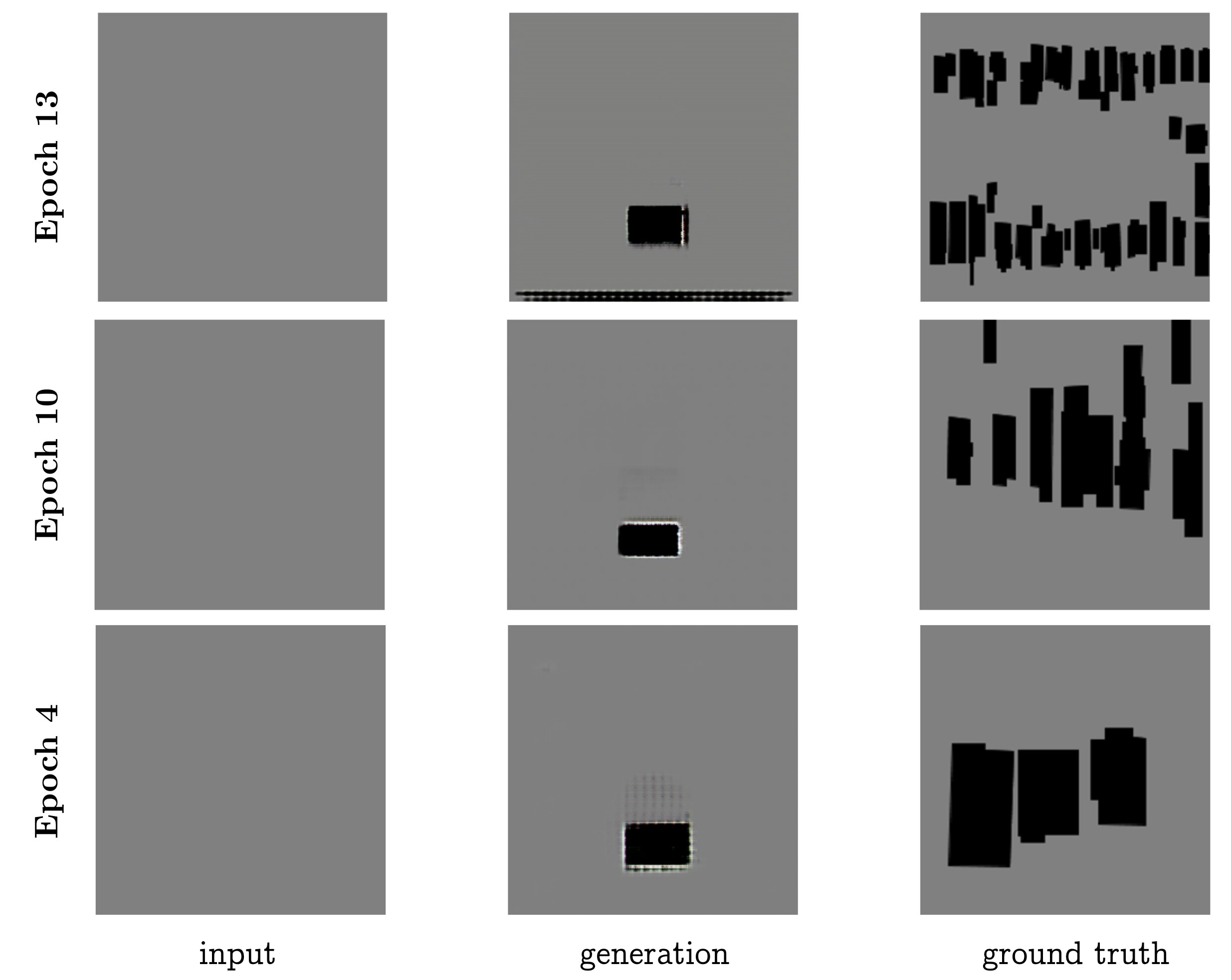
Figure 9: Task 1, experiencing possible mode collapse at a handful of earlier epochs.
Though this effect is understandable given the potential confounding inputs (all grey boxes), the model exits this behavior after more training. We would be interested in disentangling what aspect of the training helped remedy this—was it the optimization method? The discriminator “catching up” to the mode? Or simply the L1 loss?—but we would need to conduct ablations and further model analysis to propose an answer to this question.
Task 2
Similar to with task 1, the model is able to pick up on copying general background shapes over to the output by the end of epoch 1, though the results are fuzzy, and it has trouble producing buildings (Figure 10).
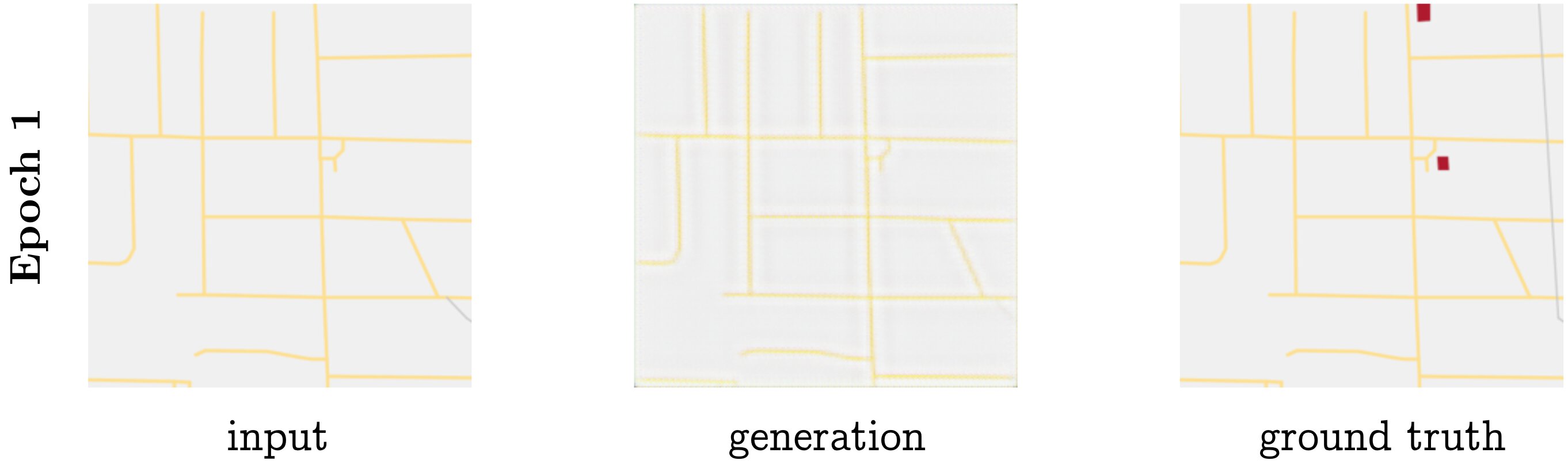
Figure 10: Task 2, after 1 epoch.
By a few dozen epochs in, the model faithfully copies over the non-building context, and generates buildings in largely the appropriate places. However, at this point it prefers larger blobs in as many spots as possible, producing cellular-looking outputs that are easily recognized as fake (Figure 11).
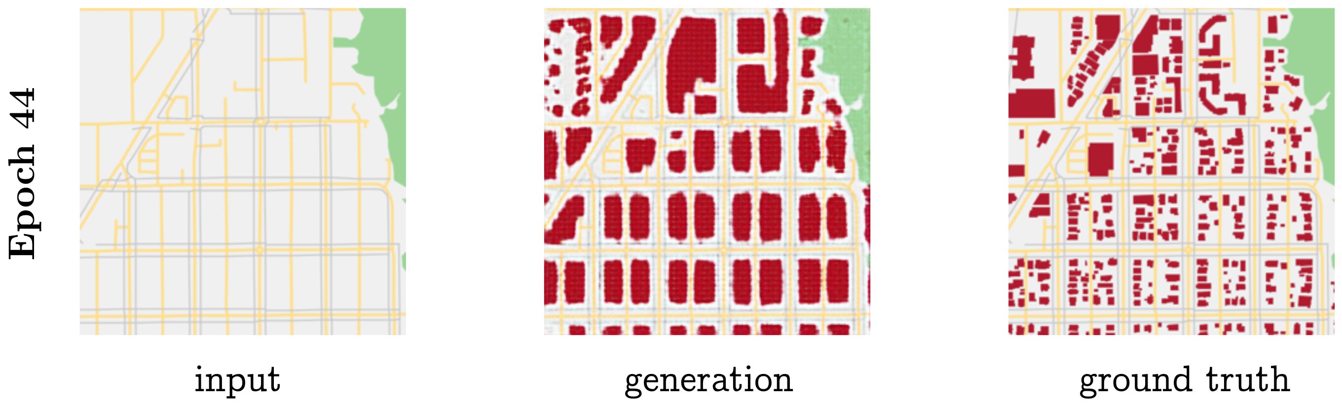
Figure 11: Task 2, after 44 epochs.
By the end of training, the model has reached generally decent performance on many of the inputs. Figure 12 shows the model after its final 200th epoch of training, generating a remarkably faithful output compared to the gold.
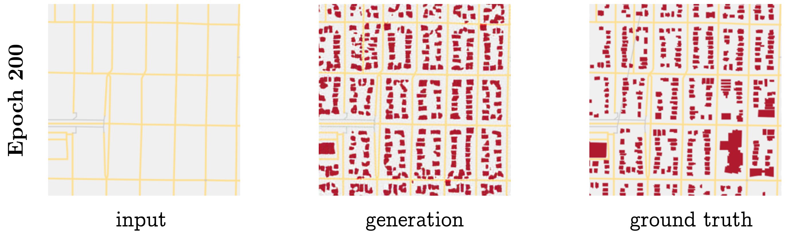
Figure 12: Task 2, the final model after 200 epochs.
Success cases
There are a few cases that the model can handle very well, shown in the three rows in Figure 13. The first row demonstrates the situation where the model excels the most: in regular, dense, suburban grids. This is likely due to the large quantity of similarly structured examples in the training set, as well as the uniformity of the output being both regular (for the model) and difficult for human eyes to distinguish (for subjective quality).
The second row shows a geographic pattern the model has learned: near parks, there are few buildings. The buildings that exist near parks are also rarely on the parks themselves (with rare exceptions being visitor centers).
The third row illustrates a seemingly trivial but interesting pattern the model has learned: that buildings do not go between freeway roads.
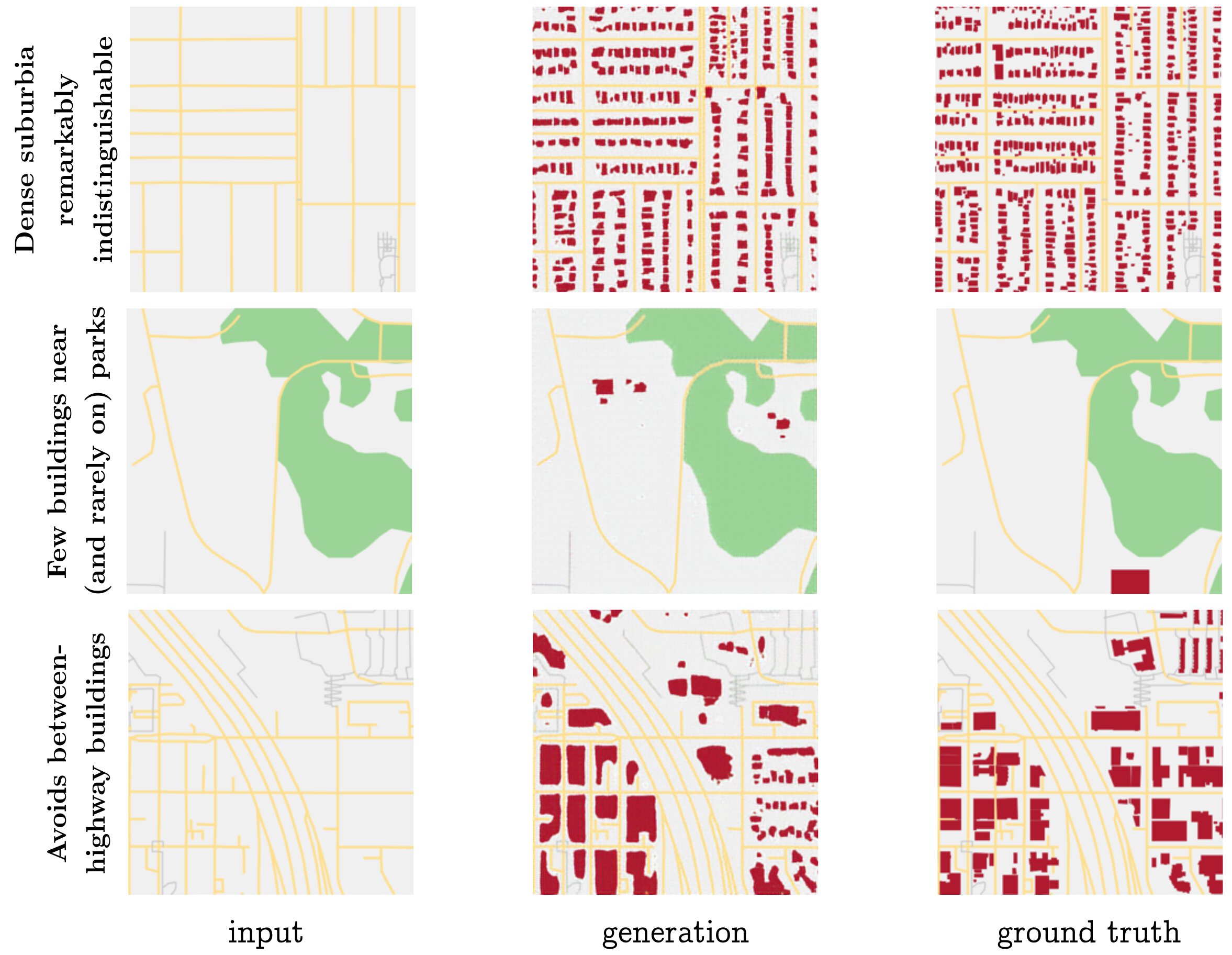
Figure 13: Task 2, three patterns the model has learned to reproduce well.
Failure cases
The model is of course not without its shortcomings. Figure 14 illustrates two of the main problems that plague the model even after it is fully trained. In the first row we see that the model still generates blobs for buildings, especially in-between curvy blocks. The second row demonstrates visual artifacts that make the model often easy to spot by human eyes: the white banding in the green park area, and the color mixtures around the long vertical grey lines.
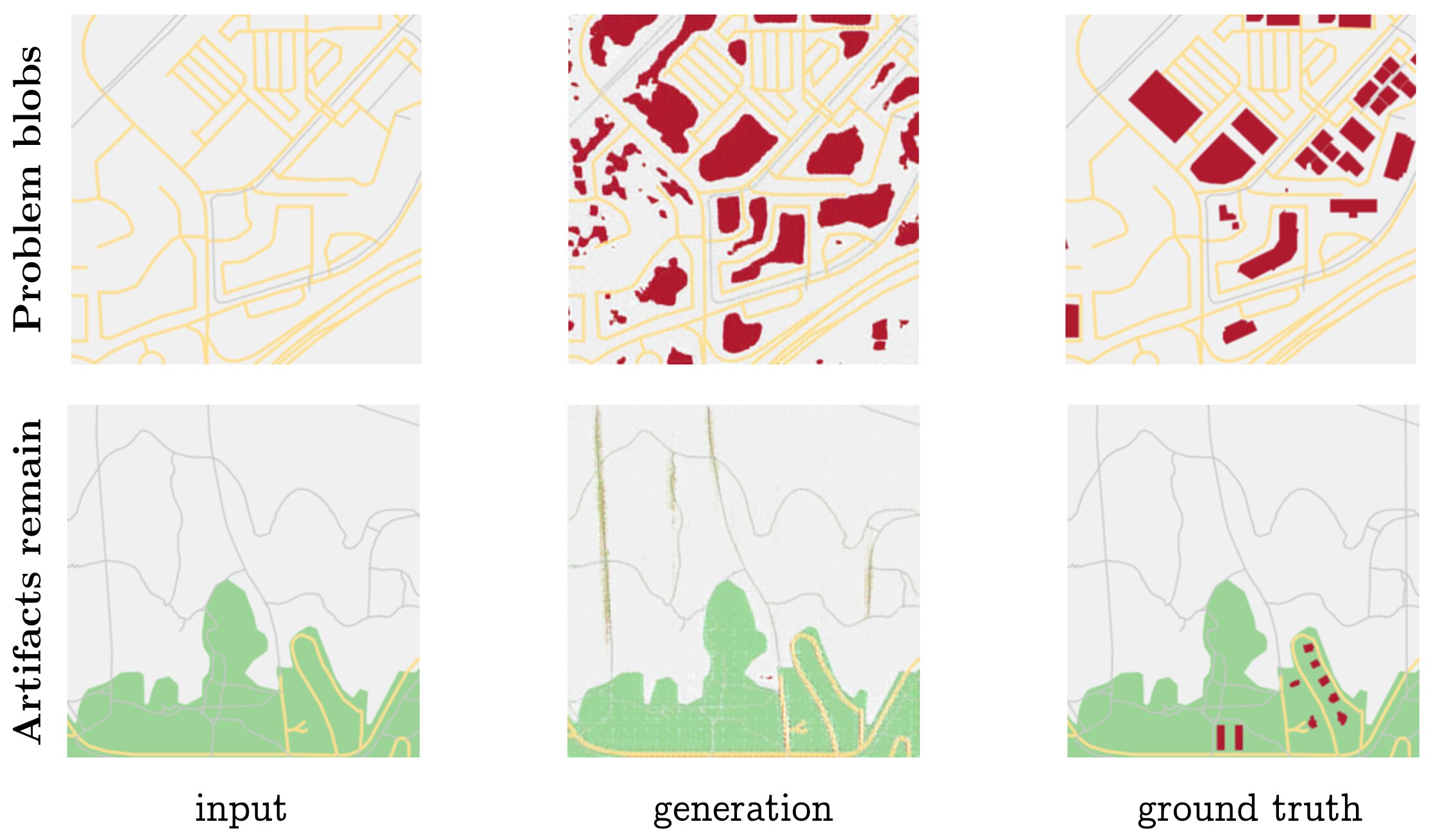
Figure 14: Task 2, two problems the model has even after training.
Unpredictable Sparsity
Some of the most frequent failures cases for the model were arguably not due to shortcomings of the model itself, but the unpredictability of the task. Figure 15 shows the sparsity / density issue happening in both directions. Some road networks, though seemingly regular and residential, in fact have no buildings in them, and so the model guesses completely wrong (first row). On the other hand, other road networks that appear to possibly be barren industrial areas near a highway are actually densely lined, and the model guesses the wrong way by leaving them empty (bottom row).
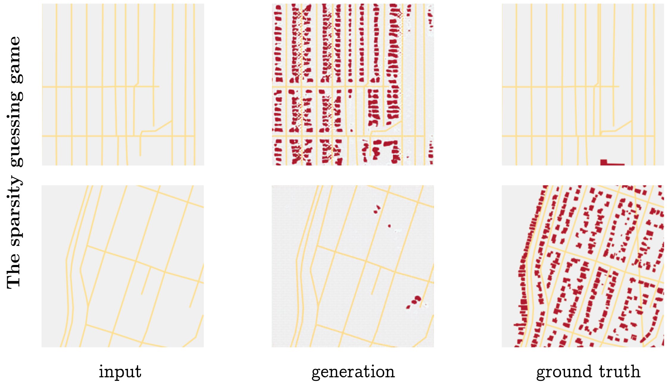
Figure 15: Task 2, sparsity (or density) that is difficult to predict.
It may be worth taking a careful pass over several more samples of the dataset to ensure that the above sparse blocks are truly empty. One possibility is that there are other geographic landmarks (such as military areas, cemetaries, or railroad tracks) that would either explain the emptiness, or provide clues for the model to better determine when it should leave regions unoccupied.
Conclusion
We presented what is, to our knowledge, the first attempt to generate urban city layouts using machine learning. We collected two “fill in the buildings” datasets by generating custom renderings from geographic data. We showed that conditional adversarial network models perform surprisingly well on both tasks, often producing plausible results even in the absence of truly sufficient information. Our code is open source, and we would happily make the data available as well upon request.
In the future, we are eager to explore two lines of work. The first natural extension is to improve the current approach. More exhaustive feature mapping would allow us to more completely capture inconsistently labeled regions like parks and waterways, and finer grained feature rendering would allow us to differentiate more waypoint types, such as freeways, arterials, and side streets. Modifying the model to account for task-specific constraints—such as that buildings have straight edges and are closed polygons—would produce even more realistic results. Training on multiple cities and observing the style differences the model picks up would be an interesting application of the work already done. And, of course, the current approach provides the road network as input; an even greater challenge would be to generate the roads as well (though this would likely move beyond the limits of the current model).
Even more exciting to us is the second line of future work, which is to learn models inspired by traditional approaches to procedural map generation: probabilistic grammars. While this approach would be less likely to produce visually impressive results as quickly as the current model, it would stay more true to the intent of procedural generation, which is to create systems that grow rather than fill in. Unsupervised grammar induction, while daunting, has precedent in natural language processing. Grammar learning would also transfer more easily to generating other features (roads, water, parks) than would the model proposed in this paper.
Footnotes
Carlos A Vanegas, Daniel G Aliaga, Peter Wonka, Pascal Müller, Paul Waddell, and Benjamin Watson. Modelling the appearance and behaviour of urban spaces. In Computer Graphics Forum, volume 29, pages 25–42. Wiley Online Library, 2010. ↩︎
Basil Weber, Pascal Müller, Peter Wonka, and Markus Gross. Interactive geometric simulation of 4d cities. In Computer Graphics Forum, volume 28, pages 481–492. Wiley Online Library, 2009. ↩︎ ↩︎
Arnaud Emilien, Adrien Bernhardt, Adrien Peytavie, Marie-Paule Cani, and Eric Galin. Procedural generation of villages on arbitrary terrains. The Visual Computer, 28(6-8):809– 818, 2012. ↩︎
Fuzhang Wu, Dong-Ming Yan, Weiming Dong, Xiaopeng Zhang, and Peter Wonka. Inverse procedural modeling of facade layouts. arXiv preprint arXiv:1308.0419, 2013. ↩︎
Ondrej Št’ava, Bedrich Beneš, Radomir Mĕch, Daniel G Aliaga, and Peter Krištof. Inverse procedural modeling by automatic generation of l-systems. In Computer Graphics Forum, volume 29, pages 665–674. Wiley Online Library, 2010. ↩︎
Lubin Fan and Peter Wonka. A probabilistic model for exteriors of residential buildings. ACM Transactions on Graphics (TOG), 35(5):155, 2016. ↩︎
Andelo Martinovic and Luc Van Gool. Bayesian grammar learning for inverse procedural modeling. In Proceedings of the IEEE Conference on Computer Vision and Pattern Recognition, pages 201–208, 2013. ↩︎
Evangelos Kalogerakis, Siddhartha Chaudhuri, Daphne Koller, and Vladlen Koltun. A probabilistic model for component-based shape synthesis. ACM Transactions on Graphics (TOG), 31(4):55, 2012. ↩︎
Alexander Toshev, Philippos Mordohai, and Ben Taskar. Detecting and parsing architecture at city scale from range data. In Computer Vision and Pattern Recognition (CVPR), 2010 IEEE Conference on, pages 398–405. IEEE, 2010. ↩︎
Daniel G Aliaga, Bedrich Beneš, Carlos A Vanegas, and Nathan Andrysco. Interactive reconfiguration of urban layouts. IEEE Computer Graphics and Applications, 28(3), 2008. ↩︎
Daniel G Aliaga, Carlos A Vanegas, and Bedrich Beneš. Interactive example-based urban layout synthesis. In ACM transactions on graphics (TOG), volume 27, page 160. ACM, 2008. ↩︎
Carlos A Vanegas, Tom Kelly, Basil Weber, Jan Halatsch, Daniel G Aliaga, and Pascal Müller. Procedural generation of parcels in urban modeling. In Computer graphics forum, volume 31, pages 681–690. Wiley Online Library, 2012. ↩︎
Gen Nishida, Ignacio Garcia-Dorado, and Daniel G Aliaga. Example-driven procedural urban roads. In Computer Graphics Forum, volume 35, pages 5–17. Wiley Online Library, 2016. ↩︎
Philip Isola, Jun-Yan Zhu, Tinghui Zhou, and Alexei A. Efros. Image-to-image translation with conditional adversarial networks. In CVPR, 2017. ↩︎
